The Definitive Guide
Jacqueline Weber
Extensive review of early reference manualAndrea Hörster
Extensive review of early reference manualKatrina Dlugosch
Draft for section on preprocessing of ESTs in EST manualMIRA Version V5rc1
Copyright © 2018 Bastien Chevreux
This documentation is licensed under the Creative Commons Attribution-NonCommercial-ShareAlike 3.0 Unported License. To view a copy of this license, visit http://creativecommons.org/licenses/by-nc-sa/3.0/ or send a letter to Creative Commons, 171 Second Street, Suite 300, San Francisco, California, 94105, USA.
Table of Contents
- Preface
- 1. Introduction to MIRA
- 2. Installing MIRA
- 3. Preparing data
- 4. Cookbook: de-novo genome assemblies
- 5. Cookbook: Mapping
- 6. Cookbook: de-novo EST / RNASeq assemblies
- 7. Working with the results of MIRA
- 8. Utilities in the MIRA package
- 9. MIRA 5 reference manual
- 10. Assembly of hard genome or EST / RNASeq projects
- 11. Description of sequencing technologies
- 12. Some advice when going into a sequencing project
- 13. Bits and pieces
- 14. Frequently asked questions
- 15. The MAF format
- 16. Log and temporary files used by MIRA
List of Figures
- 1.1. How MIRA learns from misassemblies (1)
- 1.2. How MIRA learns from misassemblies (2)
- 1.3. How MIRA learns from misassemblies (3)
- 1.4. Slides presenting the repeat locator at the GCB 99
- 1.5. Slides presenting the Edit automatic Sanger editor at the GCB 99
- 1.6. Sanger assembly without EdIt automatic editing routines
- 1.7. Sanger assembly with EdIt automatic editing routines
- 1.8. 454 assembly without 454 automatic editing routines
- 1.9. 454 assembly with 454 automatic editing routines
- 1.10. Coverage of a contig.
- 1.11. Repetitive end of a contig
- 1.12. Non-repetitive end of a contig
- 1.13. MIRA pointing out problems in hybrid assemblies (1)
- 1.14. Coverage equivalent reads (CERs) explained.
- 1.15. Coverage equivalent reads let SNPs become very visible in assembly viewers
- 1.16. SNP tags in a MIRA assembly
- 1.17. Tag pointing out a large deletion in a MIRA mapping assembly
- 7.1. Format conversions with miraconvert
- 7.2. Conversions needed for other tools.
- 7.3. Join at a repetitive site which should not be performed due to missing spanning templates.
- 7.4. Join at a repetitive site which should be performed due to spanning templates being good.
- 7.5. Pseudo-repeat in 454 data due to sequencing artifacts
- 7.6. "SROc" tag showing a SNP position in a Solexa mapping assembly.
- 7.7. "SROc" tag showing a SNP/indel position in a Solexa mapping assembly.
- 7.8. "MCVc" tag (dark red stretch in figure) showing a genome deletion in Solexa mapping assembly.
- 7.9. An IS150 insertion hiding behind a WRMc and a SRMc tags
- 7.10. A 16 base pair deletion leading to a SROc/UNsC xmas-tree
- 7.11. An IS186 insertion leading to a SROc/UNsC xmas-tree
- 11.1. The Solexa GGCxG problem.
- 11.2. The Solexa GGC problem, forward example
- 11.3. The Solexa GGC problem, reverse example
- 11.4.
A genuine place of interest almost masked by the
GGCxGproblem. - 11.5. Example for no GC coverage bias in 2008 Solexa data.
- 11.6. Example for GC coverage bias starting Q3 2009 in Solexa data.
- 11.7. Example for GC coverage bias, direct comparison 2008 / 2010 data.
- 11.8. Example for good IonTorrent data (100bp reads)
- 11.9. Example for problematic IonTorrent data (100bp reads)
- 11.10. Example for a sequencing direction dependent indel
“How much intelligence does one need to sneak upon lettuce? ” | ||
| --Solomon Short | ||
![[Note]](images/note.png) | Note |
|---|---|
A quick note at the start: I am scaling back the scope I recommend MIRA for. For genome de-novo assemblies or mapping projects, haploid organisms up to 20 to 40 megabases should be the limit. Do not use MIRA if you have PacBio or Oxford Nanopore reads. Then again, for polishing those assemblies with Illumina data, MIRA is really good. For mapping projects, do not use MIRA if you expect splicing like, e.g., RNASeq against an eukaryotic genome. Lastly, Illumina projects with more than 40 to 60 million reads start to be so resource intensive that you might be better served with other assemblers or mapping programs. I know some people use MIRA for de-novo RNASeq with 300 million reads because they think it's worth it, but they wait more than a month then for the calculation to finish. |
This "book" is actually the result of an exercise in self-defense. It contains texts from several years of help files, mails, postings, questions, answers etc.pp concerning MIRA and assembly projects one can do with it.
I never really intended to push MIRA. It started out as a PhD thesis and I subsequently continued development when I needed something to be done which other programs couldn't do at the time. But MIRA has always been available as binary on the Internet since 1999 ... and as Open Source since 2007. Somehow, MIRA seems to have caught the attention of more than just a few specialised sequencing labs and over the years I've seen an ever growing number of mails in my inbox and on the MIRA mailing list. Both from people having been "since ever" in the sequencing business as well as from labs or people just getting their feet wet in the area.
The help files -- and through them this book -- sort of reflect this development. Most of the chapters[1] contain both very specialised topics as well as step-by-step walk-throughs intended to help people to get their assembly projects going. Some parts of the documentation are written in a decidedly non-scientific way. Please excuse, time for rewriting mails somewhat lacking, some texts were re-used almost verbatim.
The last few years have seen tremendous change in the sequencing technologies and MIRA 5 reflects that: core data structures and routines had to be thrown overboard and replaced with faster and/or more versatile versions suited for the broad range of technologies and use-cases I am currently running MIRA with.
While other programs are nowadays better suited for many assembly tasks -- think SPADES for larger Illumina data sets or Falcon / Canu for PacBio -- I still regularly come back to MIRA when accuracy is important or catch the above mentioned programs doing something silly.
Nothing is perfect, and both MIRA and this documentation (even if it is rather pompously called Definitive Guide) are far from it. If you spot an error either in MIRA or this manual, feel free to report it. Or, even better, correct it if you can. At least with the manual files it should be easy: they're basically just some decorated text files.
I hope that MIRA will be as useful to you as it has been to me. Have a lot of fun with it.
Berlin, Feb 2019
Bastien Chevreux
[1] Avid readers of David Gerrold will certainly recognise the quotes from his books at the beginning of each chapter
Table of Contents
- 1.1. What is MIRA?
- 1.2. What to read in this manual and where to start reading?
- 1.3. The MIRA quick tour
- 1.4. For which data sets to use MIRA and for which not
- 1.5. Any special features I might be interested in?
- 1.5.1. MIRA learns to discern non-perfect repeats, leading to better assemblies
- 1.5.2. MIRA has integrated editors for data from Sanger, 454, IonTorrent sequencing
- 1.5.3. MIRA lets you see why contigs end where they end
- 1.5.4. MIRA tags problematic decisions in hybrid assemblies
- 1.5.5. MIRA for polishing of PacBio or ONT assemblies
- 1.5.6. MIRA allows older finishing programs to cope with amount data in Illumina mapping projects
- 1.5.7. MIRA tags SNPs and other features, outputs result files for biologists
- 1.5.8. MIRA has ... much more
- 1.6. Versions, Licenses, Disclaimer and Copyright
- 1.7. Getting help / Mailing lists / Reporting bugs
- 1.8. Author
- 1.9. Miscellaneous
“Half of being smart is to know what you're dumb at. ” | ||
| --Solomon Short | ||
MIRA is a multi-pass DNA sequence data assembler/mapper for whole genome and EST/RNASeq projects. MIRA assembles/maps reads gained by
electrophoresis sequencing (aka Sanger sequencing)
Illumina (Solexa) sequencing
Less so: 454 pyro-sequencing (GS20, FLX or Titanium)
Less so: Ion Torrent
into contiguous sequences (called contigs). One can use the sequences of different sequencing technologies either in a single assembly run (a true hybrid assembly) or by mapping one type of data to an assembly of other sequencing type (a semi-hybrid assembly (or mapping)) or by mapping a data against consensus sequences of other assemblies (a simple mapping).
The MIRA acronym stands for Mimicking Intelligent Read Assembly and the program pretty well does what its acronym says (well, most of the time anyway). It is the Swiss army knife of sequence assembly that I've used and developed during the past 20 years to get assembly jobs I work on done efficiently - and especially accurately. That is, without me actually putting too much manual work into it.
Over time, other labs and sequencing providers have found MIRA useful for assembly of extremely 'unfriendly' projects containing lots of repetitive sequences. As always, your mileage may vary.
At the last count, this manual had almost 200 pages and this might seem a little bit daunting. However, you very probably do not need to read everything.
You should read most of this introductional chapter though: e.g.,
the part with the MIRA quick tour
the part which gives a quick overview for which data sets to use MIRA and for which not
the part which showcases different features of MIRA (lots of screen shots!)
where and how to get help if things don't work out as you expected
After that, reading should depend on the type of data you intend to work with: there are specific chapters for assembly of de-novo, of mapping and of EST / RNASeq projects. They all contain an overview on how to define your data and how to launch MIRA for these data sets. There is also chapter on how to prepare data sets from specific sequencing technologies.
The chapter on working with results of MIRA should again be of general interest to everyone. It describes the structure of output directories and files and gives first pointers on what to find where. Also, converting results into different formats -- with and without filtering for specific needs -- is covered there.
As the previously cited chapters are more introductory in their nature, they do not go into the details of MIRA parametrisation. While MIRA has a comprehensive set of standard settings which should be suited for a majority of assembly tasks, the are more than 150 switches / parameters with which one can fine tune almost every aspect of an assembly. A complete description for each and every parameter and how to correctly set parameters for different use cases and sequencing technologies can be found in the reference chapter.
As not every assembly project is simple, there is also a chapter with tips on how to deal with projects which turn out to be "hard." It certainly helps if you at least skim through it even if you do not expect to have problems with your data ... it contains a couple of tricks on what one can see in result files as well as in temporary and log files which are not explained elsewhere.
MIRA comes with a number of additional utilities which are described in an own chapter. While the purpose of miraconvert should be quite clear quite quickly, the versatility of use cases for mirabait might surprise more than one. Be sure to check it out.
As from time to time some general questions on sequencing are popping up on the MIRA talk mailing list, I have added a chapter with some general musings on what to consider when going into sequencing projects. This should be in no way a replacement for an exhaustive talk with a sequencing provider, but it can give a couple of hints on what to take care of.
There is also a FAQ chapter with some of the more frequently asked questions which popped up in the past few years.
Finally, there are also chapters covering some more technical aspects of MIRA: the MAF format and structure / content of the tmp directory have own chapters.
Complete walkthroughs ... are lacking at the moment for MIRA 4. In the MIRA 3 manual I had them, but so many things have changed (at all levels: MIRA, the sequencing technologies, data repositories) that I did not have time to update them. I probably will need quite some time to write new ones. Feel free to send me some if you are inclined to help fellow scientists.
Input can be in various formats like Staden experiment (EXP), Sanger CAF, FASTA, FASTQ or PHD file. Ancillary data containing additional information helpful to the assembly as is contained in, e.g. NCBI traceinfo XML files or Staden EXP files, is also honoured. If present, base qualities in phred style and SCF signal electrophoresis trace files are used to adjudicate between or even correct contradictory stretches of bases in reads by either the integrated automatic EdIt editor (written by Thomas Pfisterer) or the assembler itself.
MIRA was conceived especially with the problem of repeats in genomic data and SNPs in transcript (EST / RNASeq) data in mind. Considerable effort was made to develop a number of strategies -- ranging from standard clone-pair size restrictions to discovery and marking of base positions discriminating the different repeats / SNPs -- to ensure that repetitive elements are correctly resolved and that misassemblies do not occur.
The resulting assembly can be written in different standard formats like CAF, Staden GAP4 directed assembly, ACE, HTML, FASTA, simple text or transposed contig summary (TCS) files. These can easily be imported into numerous finishing tools or further evaluated with simple scripts.
The aim of MIRA is to build the best possible assembly by
having a more or less full overview on the whole project at any time of the assembly, i.e. knowledge of almost all possible read-pairs in a project,
using high confidence regions (HCRs) of several aligned read-pairs to start contig building at a good anchor point of a contig, extending clipped regions of reads on a 'can be justified' basis.
using all available data present at the time of assembly, i.e., instead of relying on sequence and base confidence values only, the assembler will profit from trace files containing electrophoresis signals, tags marking possible special attributes of DNA, information on specific insert sizes of read-pairs etc.
having 'intelligent' contig objects accept or refuse reads based on the rate of unexplainable errors introduced into the consensus
learning from mistakes by discovering and analysing possible repeats differentiated only by single nucleotide polymorphisms. The important bases for discriminating different repetitive elements are tagged and used as new information.
using the possibility given by the integrated automatic editor to correct errors present in contigs (and subsequently) reads by generating and verifying complex error hypotheses through analysis of trace signals in several reads covering the same area of a consensus,
iteratively extending reads (and subsequently) contigs based on
additional information gained by overlapping read pairs in contigs and
corrections made by the automated editor.
MIRA was part of a bigger project that started at the DKFZ (Deutsches Krebsforschungszentrum, German Cancer Research Centre) Heidelberg in 1997: the "Bundesministerium für Bildung, Wissenschaft, Forschung und Technologie" supported the PhD thesis of Thomas and myself by grant number 01 KW 9611. Beside an assembler to tackle difficult repeats, the grant also supported the automated editor / finisher EdIt package -- written by Thomas Pfisterer. The strength of MIRA and EdIt is the automatic interaction of both packages which produces assemblies with less work for human finishers to be done.
I'd like to thank everybody who reported bugs to me, pointed out problems, sent ideas and suggestions they encountered while using the predecessors. Please continue to do so, the feedback made this third version possible.
As a general rule of thumb: if you have an organism with more than 100 to 150 megabases or more than 20 to 40 million reads, you might want to try other assemblers first.
For genome assembly, the version 5 series of MIRA have been reported to work on projects with something like a million Sanger reads (~80 to 100 megabases at 10x coverage), five to ten million 454 Titanium reads (~100 megabases at 20x coverage) and 20 to 40 million Illumina reads (enough for de-novo of a bacterium or a small eukaryote with 76mers to 300mers).
Provided you have the memory, MIRA is expected to work in de-novo mode with
Sanger reads: 5 to 10 million
454 reads: 5 to 15 million
Ion Torrent reads: 5 to 15 million
Illumina reads: in normal operation, up to 40 million reads. Some people use it on up to 300 million, but you'll need a really big machine and month of computation time ... I do not recommend that.
and "normal" coverages, whereas "normal" would be at no more than 50x to 70x for genome projects. Higher coverages will also work, but may create somewhat larger temporary files without heavy parametrisation. Lower coverages (<4x for Sanger, <10x for 454, < 10x for IonTorrent) also need special attention in the parameter settings.
As the complexity of mapping is a lot lower than de-novo, one can basically double (perhaps even triple) the number of reads compared to 'de-novo'. The limiting factor will be the amount of RAM though, and MIRA will also need lots of it if you go into eukaryotes.
The main limiting factor regarding time will be the number of reference sequences (backbones) you are using. MIRA being pedantic during the mapping process, it might be a rather long wait if you have more than 40 megabase of reference sequences.
The default values for MIRA should allow it to work with many EST and RNASeq data sets, sometimes even from non-normalised libraries. For extreme coverage cases however (like, something with a lot of cases at and above 10k coverage), one would perhaps want to resort to data reduction routines before feeding the sequences to MIRA.
On the other hand, recent developments of MIRA were targeted at making de-novo RNASeq assembly of non-normalised libraries liveable, and indeed I now regularly use MIRA for data sets with up to 50 million Illumina 250bp paired-end reads.
Mapping 50 to 60 million sequences against 20k to 30k gene reference sequences is doable, but slow and memory intensive.
| Note |
|---|---|
| For mapping against an eukaryotic genome: MIRA does not splice reads in mapping mode. While it is able to more or less handle insertion / deletions of up to 15% of a read length, splices larger than that will not be made: MIRA will still map the reads, but call a lot of SNPs in the parts which should have been spliced. |
A few perhaps.
| Note |
|---|---|
The screen shots in this section show data from assemblies produced with MIRA, but the visualisation itself is done in a finishing program named gap4. Some of the screen shots were edited for showing a special feature of MIRA. E.g., in the screen shots with Illumina data, quite some reads were left out of the view pane as else -- due to the amount of data -- these screen shots would need several pages for a complete printout. |
MIRA is an iterative assembler (it works in several passes) and acts a bit like a child when exploring the world: it explores the assembly space and is specifically parameterised to allow a couple of assembly errors during the first passes. But after each pass some routines (the "parents", if you like) check the result, searching for assembly errors and deduce knowledge about specific assemblies MIRA should not have ventured into. MIRA will then prevent these errors to re-occur in subsequent passes.
As an example, consider the following multiple alignment:
Figure 1.1. How MIRA learns from misassemblies (1). Multiple alignment after 1st pass with an obvious assembly error, notice the clustered columns discrepancies. Two slightly different repeats were assembled together.
 |
These kind of errors can be easily spotted by a human, but are hard to prevent by normal alignment algorithms as sometimes there's only one single base column difference between repeats (and not several as in this example).
MIRA spots these things (even if it's only a single column), tags the base positions in the reads with additional information and then will use that information in subsequent passes. The net effect is shown in the next two figures:
Figure 1.2. Multiple alignment after last pass where assembly errors from previous passes have been resolved (1st repeat site)
 |
Figure 1.3. Multiple alignment after last pass where assembly errors from previous passes have been resolved (2nd repeat site)
 |
The ability of MIRA to learn and discern non-identical repeats from each other through column discrepancies is nothing new. Here's the link to a paper from a talk I had at the German Conference on Bioinformatics in 1999: http://www.bioinfo.de/isb/gcb99/talks/chevreux/
I'm sure you'll recognise the basic principle in figures 8 and 9. The slides from the corresponding talk also look very similar to the screen shots above:

You can get the talk with these slides here: http://chevreux.org/dkfzold/gcb99/bachvortrag_gcb99.ppt
In the first versions in 1999, the EdIt automatic Sanger sequence editor from Thomas Pfisterer was integrated into MIRA.
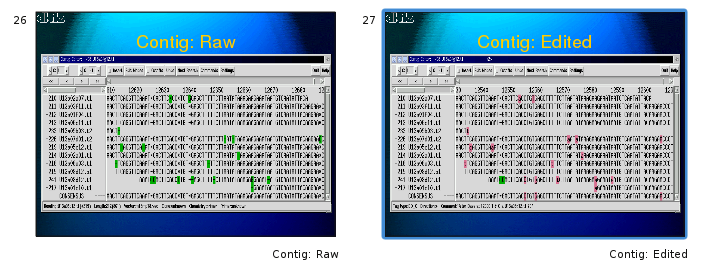
The routines used a combination of hypothesis generation/testing together with neural networks (trained on ABI and ALF traces) for signal recognition to discern between base calling errors and true multiple alignment differences. They wen back to the trace data to resolve potential conflicts and eventually recall bases using the additional information gained in a multiple alignment of reads.
Figure 1.6. Sanger assembly without EdIt automatic editing routines. The bases with blue background are base calling errors.
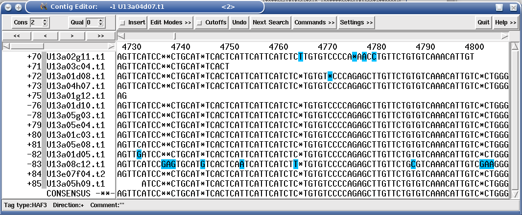 |
Figure 1.7. Sanger assembly with EdIt automatic editing routines. Bases with pink background are corrections made by EdIt after assessing the underlying trace files (SCF files in this case). Bases with blue background are base calling errors where the evidence in the trace files did not show enough evidence to allow an editing correction.
 |
With the introduction of 454 and Illumina reads, MIRA also got in 2007 specialised editors to search and correct for typical 454 and Illumina sequencing problems, like the homopolymer run over-/undercalls or the Illumina GGCxG motif problem. These editors are now integrated into MIRA itself and are not part of EdIt anymore.
While not being paramount to the assembly quality, both editors provide additional layers of safety for the MIRA learning algorithm to discern non-perfect repeats even on a single base discrepancy. Furthermore, the multiple alignments generated by these two editors are way more pleasant to look at (or automatically analyse) than the ones containing all kind of gaps, insertions, deletions etc.pp.

A very useful feature for finishing are kmer (hash) frequency tags which MIRA sets in the assembly. Provided your finishing editor understands those tags (gap4, gap5 and consed are fine but there may be others), they'll give you precious insight where you might want to be cautious when joining to contigs or where you would need to perform some primer walking. MIRA colourises the assembly with the hash frequency (HAF) tags to show repetitiveness.
You will need to read about the HAF tags in the reference manual, but in a nutshell: the HAF5, HAF6 and HAF7 tags tell you potentially have repetitive to very repetitive read areas in the genome, while HAF2 tags will tell you that these areas in the genome have not been covered as well as they should have been.
As an example, the following figure shows the coverage of a contig.

The question is now: why did MIRA stop building this contig on the left end (left oval) and why on the right end (right oval).
Looking at the HAF tags in the contig, the answer becomes quickly clear: the left contig end has HAF5 tags in the reads (shown in bright red in the following figure). This tells you that MIRA stopped because it probably could not unambiguously continue building this contig. Indeed, if you BLAST the sequence at the NCBI, you will find out that this is an rRNA area of a bacterium, of which bacteria normally have several copies in the genome:
Figure 1.11. HAF5 tags (reads shown with red background) covering a contig end show repetitiveness as reason for stopping a contig build.
 |
The right end of the same contig however ends in HAF3 tags (normal coverage, bright green in the next figure) and even HAF2 tags (below average coverage, pale green in the next image). This tells you MIRA stopped building the contig at this place simply because there were no more reads to continue. This is a perfect target for primer walking if you want to finish a genome.
Figure 1.12. HAF2 tags covering a contig end show that no more reads were available for assembly at this position.
 |
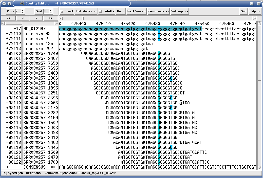
Many people combine Sanger & 454 or 454 & Illumina to improve the sequencing quality of their project through two (or more) sequencing technologies. To reduce time spent in finishing, MIRA automatically tags those bases in a consensus of a hybrid assembly where reads from different sequencing technologies severely contradict each other.
The following example shows a hybrid 454 / Illumina assembly where reads from 454 (highlighted read names in following figure) were not sure whether to have one or two "G" at a certain position. The consensus algorithm would have chosen "two Gs" for 454, obviously a wrong decision as all Illumina reads at the same spot (the reads which are not highlighted) show only one "G" for the given position. While MIRA chose to believe Illumina in this case, it tagged the position anyway in case someone chooses to check these kind of things.
Figure 1.13. A "STMS" tag (Sequencing Technology Mismatch Solved, the black square base in the consensus) showing a potentially difficult decision in a hybrid 454 / Illumina de-novo assembly.
 |
While MIRA is not really suited to assemble PacBio or Oxford Nanopore reads de-novo, it is very well suited to polish the results of such assemblies with Illumina reads in mapping projects.
TODO: example
Quality control is paramount when you do mutation analysis for biologists: I know they'll be on my doorstep the very next minute they found out one of the SNPs in the resequencing data wasn't a SNP, but a sequencing artefact. And I can understand them: why should they invest -- per SNP -- hours in the wet lab if I can invest a couple of minutes to get them data false negative rates (and false discovery rates) way below 1%? So, finishing and quality control for any mapping project is a must.
Both gap4 and consed start to have a couple of problems when projects have millions of reads: you need lots of RAM and scrolling around the assembly gets a test to your patience. Still, these two assembly finishing programs are amongst the better ones out there, although gap5 starts to quickly arrive in a state in which it allows itself to substitute to gap4.
So, MIRA reduces the number of reads in Illumina mapping projects without sacrificing information on coverage. The principle is pretty simple: for 100% matching reads, MIRA tracks coverage of every reference base and creates long synthetic, coverage equivalent reads (CERs) in exchange for the Illumina reads. Reads that do not match 100% are kept as own entities, so that no information gets lost. The following figure illustrates this:
Figure 1.14. Coverage equivalent reads (CERs) explained.
Left side of the figure: a conventional mapping with eleven reads of size 4 against a consensus (in uppercase). The inversed base in the lowest read depicts a sequencing error.
Right side of the figure: the same situation, but with coverage equivalent reads (CERs). Note that there are less reads, but no information is lost: the coverage of each reference base is equivalent to the left side of the figure and reads with differences to the reference are still present.
 |
This strategy is very effective in reducing the size of a project. As an example, in a mapping project with 9 million Illumina 36mers, MIRA created a project with 1.7m reads: 700k CER reads representing ~8 million 100% matching Illumina reads, and it kept ~950k mapped reads as they had ≥ mismatch (be it sequencing error or true SNP) to the reference. A reduction of 80%, and numbers for mapping projects with Illumina 100bp reads are in a similar range.
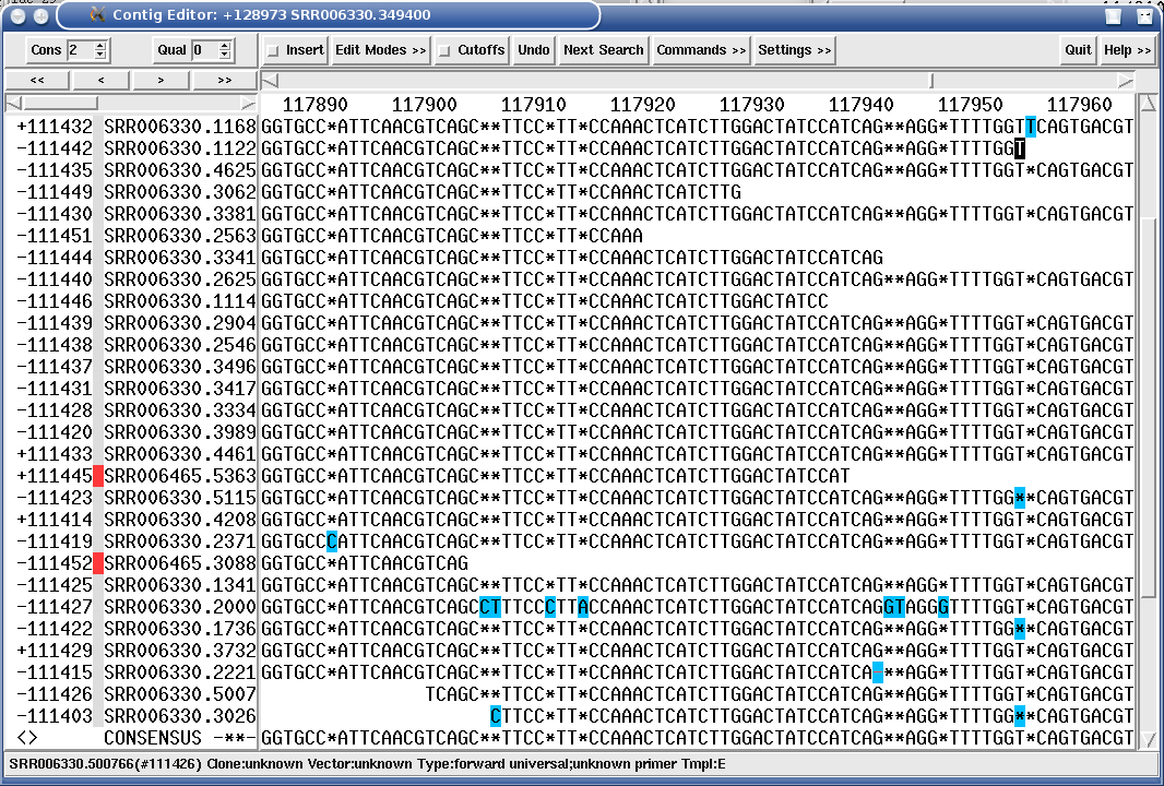
Also, mutations of the resequenced strain now really stand out in the assembly viewer as the following figure shows:

Want to assemble two or several very closely related genomes without reference, but finding SNPs or differences between them?
Tired of looking at some text output from mapping programs and guessing whether a SNP is really a SNP or just some random junk?
MIRA tags all SNPs (and other features like missing coverage etc.) it finds so that -- when using a finishing viewer like gap4 or consed -- one can quickly jump from tag to tag and perform quality control. This works both in de-novo assembly and in mapping assembly, all MIRA needs is the information which read comes from which strain.
The following figure shows a mapping assembly of Illumina 36mers against a bacterial reference sequence, where a mutant has an indel position in an gene:
Figure 1.16. "SROc" tag (Snp inteR Organism on Consensus) showing a SNP position in a Illumina mapping assembly.
 |
Other interesting places like deletions of whole genome parts are also directly tagged by MIRA and noted in diverse result files (and searchable in assembly viewers):
Figure 1.17. "MCVc" tag (Missing CoVerage in Consensus, dark red stretch in figure) showing a genome deletion in Illumina mapping assembly.
 |
| Note |
|---|---|
| For bacteria -- and if you use annotated GenBank files as reference sequence -- MIRA will also output some nice lists directly usable (in Excel) by biologists, telling them which gene was affected by what kind of SNP, whether it changes the protein, the original and the mutated protein sequence etc.pp. |
Extensive possibilities to clip data if needed: by quality, by masked bases, by A/T stretches, by evidence from other reads, ...
Routines to re-extend reads into clipped parts if multiple alignment allows for it.
Read in ancillary data in different formats: EXP, NCBI TRACEINFO XML, SSAHA2, SMALT result files and text files.
Detection of chimeric reads.
Support for many different of input and output formats (FASTA, EXP, FASTQ, CAF, MAF, ...)
Automatic memory management (when RAM is tight)
Over 150 parameters to tune the assembly for a lot of use cases, many of these parameters being tunable individually depending on sequencing technology they apply to.
There are two kind of versions for MIRA that can be compiled form source files: production and development.
Production versions are from the stable branch of the source code. These versions are available for download from SourceForge.
Development versions are from the development branch of the source tree. These are also made available to the public and should be compiled by users who want to test out new functionality or to track down bugs or errors that might arise at a given location. Release candidates (rc) also fall into the development versions: they are usually the last versions of a given development branch before being folded back into the production branch.
MIRA has been put under the GPL version 2.
This program is free software; you can redistribute it and/or modify it under the terms of the GNU General Public License as published by the Free Software Foundation; either version 2 of the License, or (at your option) any later version.
This program is distributed in the hope that it will be useful, but WITHOUT ANY WARRANTY; without even the implied warranty of MERCHANTABILITY or FITNESS FOR A PARTICULAR PURPOSE. See the GNU General Public License for more details.
You should have received a copy of the GNU General Public License along with this program; if not, write to the Free Software Foundation, Inc., 51 Franklin Street, Fifth Floor, Boston, MA 02110-1301, USA
You may also visit http://www.opensource.org/licenses/gpl-2.0.php at the Open Source Initiative for a copy of this licence.
The documentation pertaining to MIRA is licensed under the Creative Commons Attribution-NonCommercial-ShareAlike 3.0 Unported License. To view a copy of this license, visit http://creativecommons.org/licenses/by-nc-sa/3.0/ or send a letter to Creative Commons, 171 Second Street, Suite 300, San Francisco, California, 94105, USA.
© 1997-2000 Deutsches Krebsforschungszentrum Heidelberg -- Dept. of Molecular Biophysics and Bastien Chevreux (for MIRA) and Thomas Pfisterer (for EdIt)
© 2001 (and later) Bastien Chevreux.
All rights reserved.
MIRA uses the excellent Expat library to parse XML files. Expat is Copyright © 1998, 1999, 2000 Thai Open Source Software Center Ltd and Clark Cooper as well as Copyright © 2001, 2002 Expat maintainers.
See http://www.libexpat.org/ and http://sourceforge.net/projects/expat/ for more information on Expat.
Please try to find an answer to your question by first reading the documents provided with the MIRA package (FAQs, READMEs, usage guide, guides for specific sequencing technologies etc.). It's a lot, but then again, they hopefully should cover 90% of all questions.
If you have a tough nut to crack or simply could not find what you were searching for, you can subscribe to the MIRA talk mailing list and send in your question (or comment, or suggestion), see http://www.chevreux.org/mira_mailinglists.html for more information on that. Now that the number of subscribers has reached a good level, there's a fair chance that someone could answer your question before I have the opportunity or while I'm away from mail for a certain time.
| Note |
|---|---|
Please very seriously consider using the mailing list before mailing me directly. Every question which can be answered by participants of the list is time I can invest in development and documentation of MIRA. I have a day job as bioinformatician which has nothing to do with MIRA and after work hours are rare enough nowadays. Furthermore, Google indexes the mailing list and every discussion / question asked on the mailing list helps future users as they show up in Google searches. Only mail me directly (bach@chevreux.org) if you feel that there's some information you absolutely do not want to share publicly. |
| Note |
|---|---|
| Subscribing to the list before sending mails to it is necessary as messages from non-subscribers will be stopped by the system to keep the spam level low. |
To report bugs or ask for new features, please use the GitHub issue tool at: http://github.com/bachev/mira/issues. This ensures that requests do not get lost and you get the additional benefit to automatically know when a bug has been fixed as I will not send separate emails, that's what bug trackers are there for.
Finally, new or intermediate versions of MIRA will be announced on the separate MIRA announce mailing list. Traffic is very low there as the only one who can post there is me. Subscribe if you want to be informed automatically on new releases of MIRA.
Bastien Chevreux (mira): <bach@chevreux.org>
MIRA can use automatic editing routines for Sanger sequences which were
written by Thomas Pfisterer (EdIt):
<t.pfisterer@dkfz-heidelberg.de>
Please use these citations:
- For mira
Chevreux, B., Wetter, T. and Suhai, S. (1999): Genome Sequence Assembly Using Trace Signals and Additional Sequence Information. Computer Science and Biology: Proceedings of the German Conference on Bioinformatics (GCB) 99, pp. 45-56.
Chevreux, B., Pfisterer, T., Drescher, B., Driesel, A. J., Müller, W. E., Wetter, T. and Suhai, S. (2004): Using the miraEST Assembler for Reliable and Automated mRNA Transcript Assembly and SNP Detection in Sequenced ESTs. Genome Research, 14(6)
Table of Contents
- 2.1. Where to fetch MIRA
- 2.2. Installing from a precompiled binary package
- 2.3. Integration with third party programs (gap4, consed)
- 2.4. Compiling MIRA yourself
- 2.5. Installation walkthroughs
- 2.6. Compilation hints for other platforms.
- 2.7. Notes for distribution maintainers / system administrators
“A problem can be found to almost every solution. ” | ||
| --Solomon Short | ||
Source packages are usually named
mira-
miraversion.tar.bz2
| Note |
|---|---|
For
The version string sometimes can have a different format:
|
Precompiled binary packages are named in the following way:
mira_
miraversion_OS-and-binarytype.tar.bz2
| Note |
|---|---|
The
|
SourceForge: https://sourceforge.net/projects/mira-assembler/files/MIRA/
There you will normally find two directories (stable and development), both with a couple of precompiled binaries -- usually for Linux and Mac OSX -- or the source package for compiling yourself.
Examples for packages at SourceForge:
mira_4.9.8_linux-gnu_x86_64_static.tar.bz2mira_4.9.8_OSX_snowleopard_x86_64_static.tar.bz2mira-4.9.8.tar.bz2
GitHub main page: https://github.com/bachev/mira
GitHub releases (go here for binary packages): https://github.com/bachev/mira/releases
GitHub contains the live source of MIRA as well as source packages and binary packages for selected versions. Two main branches are generally interesting to the public: "master" and "development".
To get a clone of the repository on on GitHub, do:
git clone https://github.com/bachev/mira.git
cd mira
./bootstrap.sh
Once bootstrap has run through (see below for necessary prerequisites), the system is ready for a ./configure call.
The distributable package follows the one-directory-which-contains-everything-which-is-needed philosophy, but after unpacking and moving the package to its final destination, you need to run a script which will create some data files.
Download the package, unpack it.
Move the directory somewhere to your disk. Either to one of the "standard" places like, e.g.,
/opt/mira,/usr/local/miraor somewhere in your home directorySoftlink the binaries which are in the 'bin' directory into a directory which is in your shell PATH. Then have the shell reload the location of PATH binaries (either
hash -rfor sh/bash orrehashfor csh/tcsh.Alternatively, add the
bindirectory of the MIRA package to your PATH variable.Test whether the binaries are installed ok via
mirabait
	  -v
which should return with the current version you downloaded and installed.Now you need to run a script which will unpack and reformat some data needed by MIRA. That script is located in the
dbdatadirectory of the package and should be called with the name of the SLS file present in the same diretory like this:arcadia:/path/to/mirapkg$cd dbdataarcadia:/path/to/mirapkg/dbdata$ls -ldrwxr-xr-x 3 bach bach 4096 2016-03-18 14:31 mira-createsls -rwxr-xr-x 1 bach bach 2547 2015-12-14 04:33 mira-install-sls-rrna.sh -rw-r--r-- 1 bach bach 337 2016-01-01 14:50 README.txt lrwxrwxrwx 1 bach bach 10421035 2016-03-18 14:28 rfam_rrna-21-12.sls.gzarcadia:/path/to/mirapkg/dbdata$./mira-install-sls-rrna.sh rfam_rrna-21-12.sls.gzThis will take a minute or so. Then you're done for MIRA.
Additional scripts for special purposes are in the
scripts directory. You might or might not want to
have them in your $PATH.
Scripts and programs for MIRA from other authors are in the
3rdparty directory. Here too, you may or may not
want to have (some of them) in your $PATH.
MIRA sets tags in the assemblies that can be read and interpreted by the Staden gap4 package or consed. These tags are extremely useful to efficiently find places of interest in an assembly (be it de-novo or mapping), but both gap4 and consed need to be told about these tags.
Data files for a correct integration are delivered in the
support directory of the distribution. Please
consult the README in that directory for more information on how to
integrate this information in either of these packages.
| Note |
|---|---|
| As a general rule of thumb, you do NOT want to compile MIRA yourself. Fetch a precompiled binary if possible. |
Compiling the 5.x series of MIRA needs a C++14 compatible tool chain, i.e., systems starting from 2013/2014 should be OK. The requisites for compiling MIRA are:
gcc ≥ 6.1, with libstdc++6. Or clang ≥ 3.5.
You really want to use a simple installation package pre-configured for your system, but in case you want or have to install gcc or clang yourself, you will have a lot of fun.
BOOST library ≥ 1.48 (≥ 1.61 on OSX).
You really want to use a simple installation package pre-configured for your system, but in case you want or have to install BOOST yourself, please refer to http://www.boost.org/ for more information on the BOOST library.
![[Warning]](images/warning.png)
Warning Do NOT use a so called staged BOOST library, that will not work. - zlib. Should your system not have zlib installed or available as simple installation package, please see http://www.zlib.net/ for more information regarding zlib.
- GNU make. Should your system not have gmake installed or available as simple installation package, please see www.gnu.org/software/make/ for more information regarding GNU make.
- GNU flex ≥ 2.6.0. Should your system not have flex installed or available as simple installation package, please see http://flex.sourceforge.net/ for more information regarding flex.
- Expat library ≥ 2.0.1. Should your system not have the Expat library and header files already installed or available as simple installation package, you will need to download and install a yourself. Please see http://www.libexpat.org/ and http://sourceforge.net/projects/expat/ for information on how to do this.
- xxd. A small utility from the vim package.
For building the documentation, additional prerequisites are:
- help2man for manual pages
- xsltproc + docbook-xsl for HTML output
- a LaTEX system and dblatex for PDF output
When building from a GitHub checkout, additional prerequisites are a couple of additional tools:
- current automake and autoconf
- current libtool
If you're lucky, after fetching the source (and eventually calling ./bootstrap.sh if you worked from a GitHub checkout), all you need to do is basically:
arcadia:/path/to/mira-5.0.0$./configurearcadia:/path/to/mira-5.0.0$makearcadia:/path/to/mira-5.0.0$make install
This should install the following programs:
- mira
- miraconvert
- mirabait
- miramer
- miramem
Should the ./configure step fail for some reason or
another, you should get a message telling you at which step this
happens and and either install missing packages or tell
configure where it should search the packages it
did not find. See also next section or the system specific
walkthroughs in this chapter.
MIRA understands all standard autoconf configure arguments, the most
important one probably being --prefix= to tell
where you want to have MIRA installed. Please consult
./configure --help to get a full list of currently
supported arguments.
BOOST is maybe the most tricky library to get right in case it does
not come pre-configured for your system. The two main arguments for
helping to locate BOOST are
probably --with-boost=[ARG]
and --with-boost-libdir=LIB_DIR. Only if those
two fail, try using the other --with-boost-*= arguments
you will see from the ./configure help text.
The configure scripts honours the following MIRA specific arguments:
- --with-compiler=gcc/clang
-
Force the compilation to occur with the given compiler. The
default is clang on OSX systems and gcc on all other.
Note Using homebrew installed GCC on OSX compiled, but the executable did not run (no idea why). Using clang on Linux is untested atm. - --with-brew
- Automatically configure the build to be made entirely with and from software (compiler, libraries etc.) installed via Homebrew. Works perfectly on OSX, untested on Linux.
- --enable-warnings
- Enables compiler warnings, useful only for developers, not for users.
- --enable-debug
- Lets the MIRA binary contain C/C++ debug symbols.
- --enable-mirastatic
- Builds static binaries which are easier to distribute. Some platforms (like OpenSolaris) might not like this and you will get an error from the linker.
- --enable-optimisations
- Instructs the configure script to set optimisation arguments for compiling (on by default). Switching optimisations off (warning, high impact on run-time) might be interesting only for, e.g, debugging with valgrind.
- --enable-publicquietmira
- Some parts of MIRA can dump additional debug information during assembly, setting this switch to "no" performs this. Warning: MIRA will be a bit chatty, using this is not recommended for public usage.
- --enable-developmentversion
- Using MIRA with enabled development mode may lead to extra output on stdout as well as some additional data in the results which should not appear in real world data
- --enable-boundtracking
- --enable-bugtracking
- Both flags above compile in some basic checks into mira that look for sanity within some functions: Leaving this on "yes" (default) is encouraged, impact on run time is minimal
You will need to install a couple of tools and libraries before compiling MIRA. Here's the recipe:
sudo apt-get install gcc make flex
sudo apt-get install libexpat1-dev libboost-all-dev
Once this is done, you can unpack and compile MIRA. For a dynamically linked version, use:
tar xvjf mira-5.0.0.tar.bz2
cd mira-5.0.0
./configure
make && make install
For a statically linked version, just change the configure line from above into:
./configure --enable-mirastaticIn case you also want to build documentation yourself, you will need to install this in addition:
sudo apt-get install xsltproc docbook-xsl dblatexAnd building the documentation in PDF and HTML format is done like this:
make docs | Note |
|---|---|
People working on git checkouts of the MIRA source code will obviously need some more tools. Get them with this: |
| Note |
|---|---|
| This guide for OpenSUSE is outdated, but may give you clues on how to perform this on current systems. |
You will need to install a couple of tools and libraries before compiling MIRA. Here's the recipe:
sudo zypper install gcc-c++ boost-devel
sudo zypper install flex libexpat-devel zlib-devel
Once this is done, you can unpack and compile MIRA. For a dynamically linked version, use:
tar xvjf mira-5.0.0.tar.bz2
cd mira-5.0.0
./configure
make && make install
In case you also want to build documentation yourself, you will need this in addition:
sudo zypper install docbook-xsl-stylesheets dblatex | Note |
|---|---|
People working on git checkouts of the MIRA source code will obviously need some more tools. Get them with this: |
| Note |
|---|---|
| This guide for Fedora is outdated, but may give you clues on how to perform this on current systems. |
You will need to install a couple of tools and libraries before compiling MIRA. Here's the recipe:
sudo yum -y install gcc-c++ boost-devel
sudo yum install flex expat-devel vim-common zlib-devel
Once this is done, you can unpack and compile MIRA. For a dynamically linked version, use:
tar xvjf mira-5.0.0.tar.bz2
cd mira-5.0.0
./configure
make && make install
In case you also want to build documentation yourself, you will need this in addition:
sudo yum -y install docbook-xsl dblatex | Note |
|---|---|
People working on git checkouts of the MIRA source code will obviously need some more tools. Get them with this: |
These instructions are for OSX 10.14 (Mojave) and use Homebrew. There are other ways to do this (e.g., see the "compile everything from scratch"), but they are definetly more painful.
First, you will need to install the Apple XCode command line tools. This may be as easy as simply open a terminal and typing:
xcode-select --installHowever, on the machine I have, I got weird compilation errors and found https://github.com/frida/frida/issues/338#issuecomment-426777849 which told me to do this for things to work (don't ask me why, but this resolved my problems):
cd /Library/Developer/CommandLineTools/Packages/
open macOS_SDK_headers_for_macOS_10.14.pkg
Then, if you do not already have it, install Homebrew. See https://brew.sh/.
Then go on and install with homebrew the LLVM clang compiler suite and a couple of other things needed:
brew install llvm boost flex expat
To compile from a git checkout, you will also need these:
brew install autoconf automake libtool git
To build the HTML documentation, this:
brew install docbook-xsl
And to build the PDF documentation, we need MacTex (huge download, around 1 GiB, 6 GiB on disk) and the dblatex package:
brew cask install mactexpip install dblatex
Finally, if you want to build small, rudimentary man pages:
brew install help2manNow unpack MIRA, configure it and compile:
tar xvf mira-5.0.0.tar.bz2cd mira-5.0.0./configure --with-brew --enable-debugmake -j 2
That's it for the dynamic version.
For building an almost static version, we need some trickery:
configure with the --enable-mirastatic argument),
then ask the build system to create a distribution. This will launch a
toolchain at the end of which you will get a bundle which contains
everything needed to run, both on OSX and other Unix systems.
./configure --with-brew --enable-mirastatic --enable-debugmakemake distrib
This lets you build a self-contained static MIRA binary. The only prerequisite here is that you have a working gcc with the minimum version described above. Please download all necessary files (expat, flex, etc.pp) and then simply follow the script below. The only things that you will want to change are the path used and, maybe, the name of some packages in case they were bumped up a version or revision.
Contributed by Sven Klages.
## whatever path is appropriatecd## expat/home/gls/SvenTemp/installtar zxvf## flexexpat-2.0.1.tar.gzcdexpat-2.0.1./configure--prefix=/home/gls/SvenTemp/expatmake && make installcd## boost/home/gls/SvenTemp/installtar zxvfflex-2.5.35.tar.gzcdflex-2.5.35./configure--prefix=/home/gls/SvenTemp/flexmake && make install cd/home/gls/SvenTemp/flex/binln -s flex flex++ export PATH=/home/gls/SvenTemp/flex/bin:$PATHcd## mira itself/home/gls/SvenTemp/installtar zxvfboost_1_48_0.tar.gzcdboost_1_48_0./bootstrap.sh --prefix=/home/gls/SvenTemp/boost./b2 installexport CXXFLAGS="-I/home/gls/SvenTemp/flex/include" cd/home/gls/SvenTemp/installtar zxvfmira-3.4.0.1.tar.gzcdmira-3.4.0.1./configure --prefix=/home/gls/SvenTemp/mira\ --with-boost=/home/gls/SvenTemp/boost\ --with-expat=/home/gls/SvenTemp/expat\ --enable-mirastatic make && make install
In case you do not want a static binary of MIRA, but a dynamically linked version, the following script by Robert Bruccoleri will give you an idea on how to do this.
Note that he, having root rights, puts all additional software in /usr/local, and in particular, he keeps updated versions of Boost and Flex there.
#!/bin/sh -x

make distclean
oze=`find . -name "*.o" -print`
if [[ -n "$oze" ]]
then
   echo "Not clean."
   exit 1

fi

export prefix=${BUILD_PREFIX:-/usr/local}
export LDFLAGS="-Wl,-rpath,$prefix/lib"

./configure --prefix=$prefix \
           --enable-debug=yes \
           --enable-mirastatic=no \
           --with-boost-libdir=$prefix/lib \
           --enable-optimisations \
           --enable-boundtracking=yes \
           --enable-bugtracking=yes \
           --enable-extendedbugtracking=no
make
make installContributed by Thomas Vaughan
The system flex (/usr/bin/flex) is too old, but the devel/flex package from a recent pkgsrc works fine. BSD make doesn't like one of the lines in src/progs/Makefile, so use GNU make instead (available from pkgsrc as devel/gmake). Other relevant pkgsrc packages: devel/boost-libs, devel/boost-headers and textproc/expat. The configure script has to be told about these pkgsrc prerequisites (they are usually rooted at /usr/pkg but other locations are possible):
FLEX=/usr/pkg/bin/flex ./configure --with-expat=/usr/pkg --with-boost=/usr/pkgIf attempting to build a pkgsrc package of MIRA, note that the LDFLAGS passed by the pkgsrc mk files don't remove the need for the --with-boost option. The configure script complains about flex being too old, but this is harmless because it honours the $FLEX variable when writing out makefiles.
Depending on options/paramaters, the MIRA/mirabait binary may need
to load some additional data during the run. By default this data will
always be searched at this location:
LOCATION_OF_BINARY/../share/mira/...
That is: If the binary is, e.g.,
/opt/mira5/bin/mira with a softlink pointing from
/usr/local/bin/mira -> /opt/mira5/bin/mira
(because, e.g., /usr/local/bin may be by default in your
PATH variable), then the additional data will be searched in
/opt/mira5/share/mira/... and NOT in
/usr/local/share/mira/....
| Note |
|---|---|
| In short: since MIRA 4.9.6, moving the binary is not enough anymore. Take care to have the share directory in the right place, i.e., adjacent to the directory the MIRA binary lives in. |
Table of Contents
“Rome didn't fall in a day either.” | ||
| --Solomon Short | ||
Outside MIRA: transform .ab1 to .scf, perform sequencing vector clip (and cloning vector clip if used), basic quality clips.
Recommended program: gap4 (or rather pregap4) from the Staden 4 package.
Outside MIRA: convert SFF instrument from Roche to FASTQ, use sff_extract for that. In case you used "non-standard" sequencing procedures: clip away MIDs, clip away non-standard sequencing adaptors used in that project.
Outside MIRA: for heavens' sake: do NOT try to clip or trim by quality yourself. Do NOT try to remove standard sequencing adaptors yourself. Just leave Illumina data alone! (really, I mean it).
MIRA is much, much better at that job than you will probably ever be ... and I dare to say that MIRA is better at that job than 99% of all clipping/trimming software existing out there. Just make sure you use the [-CL:pec] (proposed_end_clip) option of MIRA.
| Note |
|---|---|
| The only exception to the above is if you (or your sequencing provider) used decidedly non-standard sequencing adaptors. Then it might be worthwhile to perform own adaptor clipping. But this will not be the case for 99% of all sequencing projects out there. |
Joining paired-ends: if you want to do this, feel free to use any tool which is out there (TODO: quick list). Just make sure they do not join on very short overlaps. For me, the minimum overlap is at least 17 bases, but I more commonly use at least 30.
Outside MIRA: need to convert BAM to FASTQ. Need to clip away non-standard sequencing adaptors if used in that project. Apart from that: leave the data alone.
Outside MIRA: you need to convert SRA format to FASTQ format. This is done using fastq-dump from the SRA toolkit from the NCBI. Make sure to have at least version 2.4.x of the toolkit. Last time I looked (March 2015), the software was at http://www.ncbi.nlm.nih.gov/Traces/sra/?view=software, the documentation for the whole toolkit was at http://www.ncbi.nlm.nih.gov/Traces/sra/?view=toolkit_doc, and for fastq-dump it was http://www.ncbi.nlm.nih.gov/Traces/sra/?view=toolkit_doc&f=fastq-dump
After extraction, proceed with preprocessing as described above, depending on the sequencing technology used.
For extracting Illumina data, use something like this:
arcadia:/some/path$fastq-dump -I --split-filessomefile.sra
| Note |
|---|---|
As fastq-dump unfortunately uses a pretty wasteful variant of the FASTQ format, you might want to reduce the file size for each FASTQ it produces by doing this: The above command performs an in-file replacement of unnecessary name and comments on the quality divider lines of the FASTQ. The exact translation of the sed is: do an in-file replacement (-i); starting on the third line, then every fourth line (3~4); substitute (s/); a line which starts (^); with a plus (+); and then can have any character (.); repeated any number of times including zero (*); until the end of the line ($); by just a single plus character (/+/). This alone reduces the file size of a typical Illumina data set with 100mers extracted from the SRA by about 15 to 20%. |
“The universe is full of surprises - most of them nasty.” | ||
| --Solomon Short | ||
This guide assumes that you have basic working knowledge of Unix systems, know the basic principles of sequencing (and sequence assembly) and what assemblers do.
While there are step by step instructions on how to setup your data and then perform an assembly, this guide expects you to read at some point in time
Before the assembly, Chapter 3: “Preparing data” to know what to do (or not to do) with the sequencing data before giving it to MIRA.
After the assembly, Chapter 7: “Working with the results of MIRA” to know what to do with the results of the assembly. More specifically, Section 7.1: “ MIRA output directories and files ”, Section 7.2: “ First look: the assembly info ”, Section 7.3: “ Converting results ”, Section 7.4: “ Filtering results ” and Section 7.5: “ Places of importance in a de-novo assembly ”.
And also Chapter 9: “MIRA 5 reference manual” to look up how manifest files should be written (Section 9.3.2: “ The manifest file: basics ” and Section 9.3.3: “ The manifest file: information on the data you have ” and Section 9.3.4: “ The manifest file: extended parameters ”), some command line options as well as general information on what tags MIRA uses in assemblies, files it generates etc.pp
Last but not least, you may be interested in some observations about the different sequencing technologies and the traps they may contain, see Chapter 11: “Description of sequencing technologies” for that. For advice on what to pay attention to before going into a sequencing project, have a look at Chapter 12: “Some advice when going into a sequencing project”.
This part will introduce you step by step how to get your data together for a simple de-novo assembly. I'll make up an example using an imaginary bacterium: Bacillus chocorafoliensis (or short: Bchoc). You collected the strain you want to assemble somewhere in the wild, so you gave the strain the name Bchoc_wt.
Just for laughs, let's assume you sequenced that bug with lots of more or less current sequencing technologies: Sanger, 454, Illumina, Ion Torrent and Pacific Biosciences.
You need to create (or get from your sequencing provider) the sequencing data in any supported file format. Amongst these, FASTQ and FASTA + FASTA-quality will be the most common, although the latter is well on the way out nowadays. The following walkthrough uses what most people nowadays get: FASTQ.
Create a new project directory (e.g. myProject)
and a subdirectory of this which will hold the sequencing data
(e.g. data).
arcadia:/path/tomkdir myProjectarcadia:/path/tocd myProjectarcadia:/path/to/myProject$mkdir data
Put the FASTQ data into that data directory so
that it now looks perhaps like this:
arcadia:/path/to/myProject$ls -l data-rw-r--r-- 1 bach users 263985896 2008-03-28 21:49 bchocwt_lane6.solexa.fastq
| Note |
|---|---|
I completely made up the file names above. You can name them anyway you
want. And you can have them live anywhere on the hard-disk, you do not
need to put them in this data directory. It's just
the way I do it ... and it's where the example manifest files a bit
further down in this chapter will look for the data files.
|
We're almost finished with the setup. As I like to have things neatly separated, I always create a directory called assemblies which will hold my assemblies (or different trials) together. Let's quickly do that:
arcadia:/path/to/myProject$mkdir assembliesarcadia:/path/to/myProject$mkdir assemblies/1sttrialarcadia:/path/to/myProject$cd assemblies/1sttrial
A manifest file is a configuration file for MIRA which tells it what type of assembly it should do and which data it should load. In this case we'll make a simple assembly of a genome with unpaired Illumina data
# Example for a manifest describing a genome de-novo assembly with # unpaired Illumina data # First part: defining some basic things # In this example, we just give a name to the assembly # and tell MIRA it should map a genome in accurate modeproject =# The second part defines the sequencing data MIRA should load and assemble # The data is logically divided into "readgroups" # here comes the unpaired Illumina dataMyFirstAssemblyjob =genome,denovo,accuratereadgroup =SomeUnpairedIlluminaReadsIGotFromTheLabdata =../../data/bchocwt_lane6.solexa.fastqtechnology =solexa
| Note |
|---|---|
Please look up the parameters of the manifest file in the main manual or the example manifest files in the following section. The ones above basically say: make an accurate denovo assembly of unpaired Illumina reads. |
Starting the assembly is now just a matter of a simple command line:
arcadia:/path/to/myProject/assemblies/1sttrial$miramanifest.conf >&log_assembly.txt
For this example - if you followed the walk-through on how to prepare the data - everything you might want to adapt in the first time are the following thing in the manifest file: options:
project= (for naming your assembly project)
Of course, you are free to change any option via the extended parameters, but this is the topic of another part of this manual.
This section will introduce you to manifest files for different use cases. It should cover the most important uses, but as always you are free to mix and match the parameters and readgroup definitions to suit your specific needs.
Taking into account that there may be a lot of combinations of sequencing technologies, sequencing libraries (shotgun, paired-end, mate-pair, etc.) and input file types (FASTQ, FASTA, GenBank, GFF3, etc.pp), the example manifest files just use Illumina and 454 as technologies, GFF3 as input file type for the reference sequence, FASTQ as input type for sequencing data ... and they do not show the multitude of more advanced features like, e.g., using ancillary clipping information in XML files, ancillary masking information in SSAHA2 or SMALT files etc.pp.
I'm sure you will be able to find your way by scanning through the corresponding section on manifest files in the reference chapter :-)
Well, we've seen that already in the section above, but here it is again ... but this time with 454 data.
# Example for a manifest describing a denovo assembly with # unpaired 454 data # First part: defining some basic things # In this example, we just give a name to the assembly # and tell MIRA it should map a genome in accurate modeproject =# The second part defines the sequencing data MIRA should load and assemble # The data is logically divided into "readgroups" # here's the 454 dataMyFirstAssemblyjob =genome,denovo,accuratereadgroup =SomeUnpaired454ReadsIGotFromTheLabdata =../../data/some454data.fastqtechnology =454
Hybrid de-novo assemblies follow the general manifest scheme: tell what you want in the first part, then simply add as separate readgroup the information MIRA needs to know to find the data and off you go. Just for laughs, here's a manifest for 454 shotgun with Illumina shotgun
# Example for a manifest describing a denovo assembly with # shotgun 454 and shotgun Illumina data # First part: defining some basic things # In this example, we just give a name to the assembly # and tell MIRA it should map a genome in accurate modeproject =# The second part defines the sequencing data MIRA should load and assemble # The data is logically divided into "readgroups" # now the shotgun 454 dataMyFirstAssemblyjob =genome,denovo,accuratereadgroup =# now the shotgun Illumina dataDataForShotgun454data =../../data/project454data.fastqtechnology =454readgroup =DataForShotgunIlluminadata =../../data/someillumina.fastqtechnology =solexa
When using paired-end data, you should know
the orientation of the reads toward each other. This is specific to sequencing technologies and / or the sequencing library preparation.
at which distance these reads should be. This is specific to the sequencing library preparation and the sequencing lab should tell you this.
In case you do not know one (or any) of the above, don't panic! MIRA is able to estimate the needed values during the assembly if you tell it to.
The following manifest shows you the most laziest way to define a paired data set by simply adding autopairing as keyword to a readgroup (using Illumina just as example):
# Example for a lazy manifest describing a denovo assembly with # one library of paired reads # First part: defining some basic things # In this example, we just give a name to the assembly # and tell MIRA it should map a genome in accurate modeproject =# The second part defines the sequencing data MIRA should load and assemble # The data is logically divided into "readgroups" # now the Illumina paired-end dataMyFirstAssemblyjob =genome,denovo,accuratereadgroup =DataIlluminaPairedLibautopairingdata =../../data/project_1.fastq ../../data/project_2.fastqtechnology =solexa
If you know the orientation of the reads and/or the library size, you can tell this MIRA the following way (just showing the readgroup definition here):
readgroup = DataIlluminaPairedEnd500Lib
data = ../../data/project_1.fastq ../../data/project_2.fastq
technology = solexa
template_size = 250 750
segment_placement = ---> <---
In cases you are not 100% sure about, e.g., the size of the DNA template, you can also give a (generous) expected range and then tell MIRA to automatically refine this range during the assembly based on real, observed distances of read pairs. Do this with autorefine modifier like this:
template_size = 50 1000 autorefineThe following manifest file is an example for assembling with several different libraries from different technologies. Do not forget you can use autopairing or autorefine :-)
# Example for a manifest describing a denovo assembly with # several kinds of sequencing libraries # First part: defining some basic things # In this example, we just give a name to the assembly # and tell MIRA it should map a genome in accurate modeproject =# The second part defines the sequencing data MIRA should load and assemble # The data is logically divided into "readgroups" # now the Illumina paired-end dataMyFirstAssemblyjob =genome,denovo,accuratereadgroup =# now the Illumina mate-pair dataDataIlluminaForPairedEnd500bpLibdata =../../data/project500bp-1.fastq ../../data/project500bp-2.fastqtechnology =solexastrain =bchoc_se1template_size =250 750segment_placement =---> <---readgroup =# some Sanger data (6kb library)DataIlluminaForMatePair3kbLibdata =../../data/project3kb-1.fastq ../../data/project3kb-2.fastqtechnology =solexastrain =bchoc_se1template_size =2500 3500segment_placement =<--- --->readgroup =# some 454 dataDataForSanger6kbLibdata =../../data/sangerdata.fastqtechnology =sangertemplate_size =5500 6500segment_placement =---> <---readgroup =# some Ion Torrent dataDataFo454Pairsdata =../../data/454data.fastqtechnology =454template_size =8000 1200segment_placement =2---> 1--->readgroup =DataFoIonPairsdata =../../data/iondata.fastqtechnology =iontortemplate_size =1000 300segment_placement =2---> 1--->
MIRA will make use of ancillary information present in the manifest file. One of these is the information to which strain (or organism or cell line etc.pp) the generated data belongs.
You just need to tell in the manifest file which data comes from which strain. Let's assume that in the example from above, the "lane6" data were from a first mutant named bchoc_se1 and the "lane7" data were from a second mutant named bchoc_se2. Here's the manifest file you would write then:
# Example for a manifest describing a de-novo assembly with # unpaired Illumina data, but from multiple strains # First part: defining some basic things # In this example, we just give a name to the assembly # and tell MIRA it should map a genome in accurate modeproject =# The second part defines the sequencing data MIRA should load and assemble # The data is logically divided into "readgroups" # now the Illumina dataMyFirstAssemblyjob =genome,denovo,accuratereadgroup =DataForSE1data =../../data/bchocse_lane6.solexa.fastqtechnology =solexastrain =bchoc_se1readgroup =DataForSE2data =../../data/bchocse_lane7.solexa.fastqtechnology =solexastrain =bchoc_se2
| Note |
|---|---|
| While assembling de-novo with multiple strains is possible, the interpretation of results may become a bit daunting in some cases. For many scenarios it might therefore be preferable to successively use the data sets in own assemblies or mappings. |
This strain information for each readgroup is really the only change you need to perform to tell MIRA everything it needs for handling strains.
Table of Contents
“You have to know what you're looking for before you can find it.” | ||
| --Solomon Short | ||
This guide assumes that you have basic working knowledge of Unix systems, know the basic principles of sequencing (and sequence assembly) and what assemblers do.
While there are step by step instructions on how to setup your data and then perform an assembly, this guide expects you to read at some point in time
Before the mapping, Chapter 3: “Preparing data” to know what to do (or not to do) with the sequencing data before giving it to MIRA.
Generally, the Chapter 7: “Working with the results of MIRA” to know what to do with the results of the assembly. More specifically, Section 7.3: “ Converting results ” Section 7.6: “ Places of interest in a mapping assembly ” Section 7.7: “ Post-processing mapping assemblies ”
And also Chapter 9: “MIRA 5 reference manual” to look up how manifest files should be written (Section 9.3.2: “ The manifest file: basics ” and Section 9.3.3: “ The manifest file: information on the data you have ” and Section 9.3.4: “ The manifest file: extended parameters ”), some command line options as well as general information on what tags MIRA uses in assemblies, files it generates etc.pp
Last but not least, you may be interested in some observations about the different sequencing technologies and the traps they may contain, see Chapter 11: “Description of sequencing technologies” for that. For advice on what to pay attention to before going into a sequencing project, have a look at Chapter 12: “Some advice when going into a sequencing project”.
This part will introduce you step by step how to get your data together for a simple mapping assembly.
I'll make up an example using an imaginary bacterium: Bacillus chocorafoliensis (or short: Bchoc).
In this example, we assume you have two strains: a wild type strain of Bchoc_wt and a mutant which you perhaps got from mutagenesis or other means. Let's imagine that this mutant needs more time to eliminate a given amount of chocolate, so we call the mutant Bchoc_se ... SE for slow eater
You wanted to know which mutations might be responsible for the observed behaviour. Assume the genome of Bchoc_wt is available to you as it was published (or you previously sequenced it), so you resequenced Bchoc_se with Solexa to examine mutations.
You need to create (or get from your sequencing provider) the sequencing data in either FASTQ or FASTA + FASTA quality format. The following walkthrough uses what most people nowadays get: FASTQ.
Create a new project directory (e.g. myProject) and a subdirectory of this which will hold the sequencing data (e.g. data).
arcadia:/path/tomkdir myProjectarcadia:/path/tocd myProjectarcadia:/path/to/myProject$mkdir data
Put the FASTQ data into that data directory so that it now looks perhaps like this:
arcadia:/path/to/myProject$ls -l data-rw-r--r-- 1 bach users 263985896 2008-03-28 21:49 bchocse_lane6.solexa.fastq -rw-r--r-- 1 bach users 264823645 2008-03-28 21:51 bchocse_lane7.solexa.fastq
| Note |
|---|---|
I completely made up the file names above. You can name them anyway you
want. And you can have them live anywhere on the hard disk, you do not
need to put them in this data directory. It's just
the way I do it ... and it's where the example manifest files a bit further down
in this chapter will look for the data files.
|
The reference sequence (the backbone) can be in a number of different formats: GFF3, GenBank (.gb, .gbk, .gbf, .gbff), MAF, CAF, FASTA. The first three have the advantage of being able to carry additional information like, e.g., annotation. In this example, we will use a GFF3 file like the ones one can download from the NCBI.
| Note |
|---|---|
| TODO: Write why GFF3 is better and where to get them at the NCBI. |
So, let's assume that our wild type
strain is in the following file:
NC_someNCBInumber.gff3.
You do not need to copy the reference sequence to your directory, but I normally copy also the reference file into the directory with my data as I want to have, at the end of my work, a nice little self-sufficient directory which I can archive away and still be sure that in 10 years time I have all data I need together.
arcadia:/path/to/myProject$cp /somewhere/NC_someNCBInumber.gff3 dataarcadia:/path/to/myProject$ls -l data-rw-r--r-- 1 bach users 6543511 2008-04-08 23:53 NC_someNCBInumber.gff3 -rw-r--r-- 1 bach users 263985896 2008-03-28 21:49 bchocse_lane6.solexa.fastq -rw-r--r-- 1 bach users 264823645 2008-03-28 21:51 bchocse_lane7.solexa.fastq
We're almost finished with the setup. As I like to have things neatly separated, I always create a directory called assemblies which will hold my assemblies (or different trials) together. Let's quickly do that:
arcadia:/path/to/myProject$mkdir assembliesarcadia:/path/to/myProject$mkdir assemblies/1sttrialarcadia:/path/to/myProject$cd assemblies/1sttrial
A manifest file is a configuration file for MIRA which tells it what type of assembly it should do and which data it should load. In this case we have unpaired sequencing data which we want to map to a reference sequence, the manifest file for that is pretty simple:
# Example for a manifest describing a mapping assembly with # unpaired Illumina data # First part: defining some basic things # In this example, we just give a name to the assembly # and tell MIRA it should map a genome in accurate modeproject =# The second part defines the sequencing data MIRA should load and assemble # The data is logically divided into "readgroups" # first, the reference sequenceMyFirstMappingjob =genome,mapping,accuratereadgroup is_reference data =# now the Illumina data../../data/NC_someNCBInumber.gff3strain =bchoc_wtreadgroup =SomeUnpairedIlluminaReadsIGotFromTheLabdata =../../data/*fastqtechnology =solexastrain =bchoc_se
| Note |
|---|---|
Please look up the parameters of the manifest file in the main manual or the example manifest files in the following section. The ones above basically say: make an accurate mapping of Solexa reads against a genome; in one pass; the name of the backbone strain is 'bchoc_wt'; the data with the backbone sequence (and maybe annotations) is in a specified GFF3 file; for Solexa data: assign default strain names for reads which have not loaded ancillary data with strain info and that default strain name should be 'bchoc_se'. |
Starting the assembly is now just a matter of a simple command line:
arcadia:/path/to/myProject/assemblies/1sttrial$miramanifest.conf >&log_assembly.txt
For this example - if you followed the walk-through on how to prepare the data - everything you might want to adapt in the first time are the following thing in the manifest file: options:
project= (for naming your assembly project)
strain_name= to give the names of your reference and mapping strain
Of course, you are free to change any option via the extended parameters, but this is the topic of another part of this manual.
This section will introduce you to manifest files for different use cases. It should cover the most important uses, but as always you are free to mix and match the parameters and readgroup definitions to suit your specific needs.
Taking into account that there may be a lot of combinations of sequencing technologies, sequencing libraries (shotgun, paired-end, mate-pair, etc.) and input file types (FASTQ, FASTA, GenBank, GFF3, etc.pp), the example manifest files just use Illumina and 454 as technologies, GFF3 as input file type for the reference sequence, FASTQ as input type for sequencing data ... and they do not show the multitude of more advanced features like, e.g., using ancillary clipping information in XML files, ancillary masking information in SSAHA2 or SMALT files etc.pp.
I'm sure you will be able to find your way by scanning through the corresponding section on manifest files in the reference chapter :-)
Well, we've seen that already in the section above, but here it is again ... this time with Ion Torrent data though.
# Example for a manifest describing a mapping assembly with # unpaired Ion data # First part: defining some basic things # In this example, we just give a name to the assembly # and tell MIRA it should map a genome in accurate modeproject =# The second part defines the sequencing data MIRA should load and assemble # The data is logically divided into "readgroups" # first, the reference sequenceMyFirstMappingjob =genome,mapping,accuratereadgroup is_reference data =# now the Ion Torrent data../../data/NC_someNCBInumber.gff3strain =bchoc_wtreadgroup =SomeUnpairedIonReadsIGotFromTheLabdata =../../data/someiondata.fastqtechnology =iontorstrain =bchoc_se
When using paired-end data in mapping, you must decide whether you want
use the MIRA feature to create long 'coverage equivalent reads' (CERs) which saves a lot of memory (both in the assembler and later on in an assembly editor). However, you then loose information about read pairs!
or whether you want to keep information about read pairs at the expense of larger memory requirements both in MIRA and in assembly finishing tools or viewers afterwards.
or a mix of the two above
The Illumina pipeline generally normally gives you two files for paired-end
data: a project-1.fastq and
project-2.fastq. The first file containing the
first read of a read-pair, the second file the second read. Depending
on the preprocessing pipeline of your sequencing provider, the names
of the reads are either the very same in both files or already have
a /1 or /2 appended. Also, your
sequencing provider may give you one big file where the reads from
both ends are present.
| Note |
|---|---|
MIRA can read all FASTQ variants produced by various Illumina pipelines, be they with or without the /1 and /2 already appended to the names. You generally do not need to do any name mangling before feeding the data to MIRA. However, MIRA will shell out a warning if read names are longer than 40 characters. |
When using paired-end data, you should know
the orientation of the reads toward each other. This is specific to sequencing technologies and / or the sequencing library preparation.
at which distance these reads should be. This is specific to the sequencing library preparation and the sequencing lab should tell you this.
In case you do not know one (or any) of the above, don't panic! MIRA is able to estimate the needed values during the assembly if you tell it to.
The following manifest shows you the most laziest way to define a paired data set by simply adding autopairing as keyword to a readgroup (using Illumina just as example):
# Example for a lazy manifest describing a mapping assembly with # one library of paired reads # First part: defining some basic things # In this example, we just give a name to the assembly # and tell MIRA it should map a genome in accurate modeproject =# The second part defines the sequencing data MIRA should load and assemble # The data is logically divided into "readgroups" # first the reference sequenceMyFirstMappingjob =genome,mapping,accuratereadgroup is_reference data =# now the Illumina paired-end data../../data/NC_someNCBInumber.gff3strain =bchoc_wtreadgroup =DataIlluminaPairedLibautopairingdata =../../data/project_1.fastq ../../data/project_2.fastqtechnology =solexastrain =bchoc_se1
See? Wasn't hard and it did not hurt, did it? One just needs to tell MIRA it should expect paired reads via the autopairing keyword and that is everything you need.
If you are lazy, or want to efficiently include multiple FASTQ files, you can use regular expressions in the line which defines the data to load. E.g., if there were only two FASTQ files in the directory named _1 and _2, you can write this:
data = ../../data/project_?.fastqNotice the question mark in the above line? Read more about how to use this and other shortcuts in Section 9.3.3.2: “ Defining data files to load ”
If you know the orientation of the reads and/or the library size, you can tell this MIRA the following way (just showing the readgroup definition here):
readgroup = DataIlluminaPairedEnd500Lib
data = ../../data/project_1.fastq ../../data/project_2.fastq
technology = solexa
template_size = 250 750
segment_placement = ---> <---
In cases you are not 100% sure about, e.g., the size of the DNA template, you can also give a (generous) expected range and then tell MIRA to automatically refine this range during the assembly based on real, observed distances of read pairs. Do this with autorefine modifier like this:
template_size = 50 1000 autorefineThe following manifest file is an example for mapping a 500 bp paired-end and a 3kb mate-pair library of a strain called bchoc_se1 against a GenBank reference file containing a strain called bchoc_wt:
# Example for a manifest describing a mapping assembly with # paired Illumina data, not merging reads and therefore keeping # all pair information # First part: defining some basic things # In this example, we just give a name to the assembly # and tell MIRA it should map a genome in accurate mode # As special parameter, we want to switch off merging of Solexa readsproject =# The second part defines the sequencing data MIRA should load and assemble # The data is logically divided into "readgroups" # first, the reference sequenceMyFirstMappingjob =genome,mapping,accurateparameters =SOLEXA_SETTINGS -CO:msr=noreadgroup is_reference data =# now the Illumina data../../data/NC_someNCBInumber.gff3strain =bchoc_wtreadgroup =DataForPairedEnd500bpLibautopairingdata =../../data/project500bp-1.fastq ../../data/project500bp-2.fastqtechnology =solexastrain =bchoc_se1readgroup =DataForMatePair3kbLibdata =../../data/project3kb-1.fastq ../../data/project3kb-2.fastqtechnology =solexastrain =bchoc_se1template_size =2000 4000 autorefinesegment_placement =<--- --->
Please look up the parameters used in the main manual. The ones above basically say: make an accurate mapping of Solexa reads against a genome. Additionally do not merge short short Solexa reads to the contig.
For the paired-end library, be lazy and let MIRA find out everything it needs. However, that information should be treated as "information only" by MIRA, i.e., it is not used for deciding whether a pair is well mapped.
For the mate-pair library, assume a DNA template template size of 2000 to 4000 bp (but let MIRA automatically refine this using observed distances) and the segment orientation of the read pairs follows the reverse / forward scheme. That information should be treated as "information only" by MIRA, i.e., it is not used for deciding whether a pair is well mapped.
Comparing this manifest with a manifest for unpaired-data, two parameters were added in the section for Solexa data:
-CO:msr=notells MIRA not to merge reads that are 100% identical to the backbone. This also allows to keep the template information (distance and orientation) for the reads.template_sizetells MIRA at which distance the two reads should normally be placed from each other.segment_placementtells MIRA how the different segments (reads) of a DNA template have to be ordered to form a valid representation of the sequenced DNA.
| Note |
|---|---|
Note that in mapping assemblies, these
|
| Warning |
|---|---|
If template size and segment placement checking were on, the following would happen at, e.g. sites of re-arrangement: MIRA would map the first read of a read-pair without problem. However, it would very probably reject the second read because it would not map at the specified distance or orientation from its partner. Therefore, in mapping assemblies with paired-end data, checking of the template size must be switched off to give post-processing programs a chance to spot re-arrangements. |
I'm sure you'll have picked up the general scheme of manifest files by now. Hybrid mapping assemblies follow the general scheme: simply add as separate readgroup the information MIRA needs to know to find the data and off you go. Just for laughs, here's a manifest for 454 shotgun with Illumina paired-end
# Example for a manifest describing a mapping assembly with # shotgun 454 and paired-end Illumina data, not merging reads and therefore keeping # all pair information # First part: defining some basic things # In this example, we just give a name to the assembly # and tell MIRA it should map a genome in accurate mode # As special parameter, we want to switch off merging of Solexa readsproject =# The second part defines the sequencing data MIRA should load and assemble # The data is logically divided into "readgroups" # first, the reference sequenceMyFirstMappingjob =genome,mapping,accurateparameters =SOLEXA_SETTINGS -CO:msr=noreadgroup is_reference data =# now the shotgun 454 data../../data/NC_someNCBInumber.gff3strain =bchoc_wtreadgroup =# now the paired-end Illumina dataDataForShotgun454data =../../data/project454data.fastqtechnology =454strain =bchoc_se1readgroup =DataForPairedEnd500bpLibdata =../../data/project500bp-1.fastq ../../data/project500bp-2.fastqtechnology =solexastrain =bchoc_se1template_size =250 750segment_placement =---> <---
MIRA will make use of ancillary information present in the manifest file. One of these is the information to which strain (or organism or cell line etc.pp) the generated data belongs.
You just need to tell in the manifest file which data comes from which strain. Let's assume that in the example from above, the "lane6" data were from a first mutant named bchoc_se1 and the "lane7" data were from a second mutant named bchoc_se2. Here's the manifest file you would write then:
# Example for a manifest describing a mapping assembly with # unpaired Illumina data # First part: defining some basic things # In this example, we just give a name to the assembly # and tell MIRA it should map a genome in accurate modeproject =# The second part defines the sequencing data MIRA should load and assemble # The data is logically divided into "readgroups" # first, the reference sequenceMyFirstMappingjob =genome,mapping,accuratereadgroup is_reference data =# now the Illumina data../../data/NC_someNCBInumber.gff3strain =bchoc_wtreadgroup =DataForSE1data =../../data/bchocse_lane6.solexa.fastqtechnology =solexastrain =bchoc_se1readgroup =DataForSE2data =../../data/bchocse_lane7.solexa.fastqtechnology =solexastrain =bchoc_se2
| Note |
|---|---|
| While mapping (or even assembling de-novo) with multiple strains is possible, the interpretation of results may become a bit daunting in some cases. For many scenarios it might therefore be preferable to successively use the data sets in own mappings or assemblies. |
This strain information for each readgroup is really the only change you need to perform to tell MIRA everything it needs for handling strains.
For bacteria you can map EST / RNASeq data against any reference sequence(s), be it a genome reference or transcriptome reference.
For eukaryotes, I recommend mapping against transcriptome sequences only as MIRA does not handle splice sites very well. You can get away mapping RNASeq data against 'simple' eukaryotes which have very few and small introns, like S. cerevisiae or simple fungi; but just note that the expression level for exons near larger introns will be slightly lower than the rest of the gene.
| Note |
|---|---|
The standard MIRA parameters are geared towards handling difficult mapping cases where the reference sequence can be quite different to what is actually mapped against it (10% average difference, up to 15% locally). If the data you are mapping is actually from a strain which is very similar to your reference (give or take a couple of SNPs, genome reorganisations and / or insertions and deletions), you can save a lot of time in the mapping process by relaxing a few parameters like [-SK:kms=(high-value)], [-SB:bnb=no], [-FM:mte=(low-value)]. |
Here's a very simple, albeit powerful manifest which will allow you to retrieve both SNPs and feature coverage data from the mapping results:
# Example for a lazy manifest describing a mapping assembly with # one library of paired reads # First part: defining some basic things # In this example, we just give a name to the assembly # and tell MIRA it should map EST / RNASeq data in accurate mode # Accurate mode may be "too good" for mapping, see next exampleproject =# The second part defines the sequencing data MIRA should load and assemble # The data is logically divided into "readgroups" # first the reference sequenceMyFirstMappingjob =est,mapping,accuratereadgroup is_reference data =# now the Illumina data../../data/NC_someNCBInumber.gff3strain =bchoc_wtreadgroup data =../../data/project_1.fastq ../../data/project_2.fastqtechnology =solexastrain =bchoc_se1
If you compare the above manifest to a manifest for a simple genome mapping, the only line which really changed is the job=... line, which changed from genome,mapping,accurate to est,mapping,accurate
As already alluded to, the standard MIRA mapping parameters are made to find almost anything that maps, and that takes time. In case you are mapping data which is very closely related to the reference sequence you are using, you can save time by changing the manifest slightly. Start it like this:
# Example for a lazy manifest describing a mapping assembly with # one library of paired reads which is close to your reference sequence # First part: defining some basic thingsproject =# Accurate mode may be "too good" for mapping, therefore these parameters to # speed up thingsMyFirstMappingjob =est,mapping,accurateparameters = -SK:kms=20 SOLEXA_SETTINGS -SB:bnb=no -FM:mte=6 # remaining manifest as above # ...
There are a few things to consider when using reference sequences:
MIRA is not really made to handle a big amount of reference sequences as they currently need inane amounts of memory. Use other programs for mapping against more than, say, 200 megabases.
Reference sequences can be as long as needed! They are not subject to normal read length constraints of a maximum of 32k bases. That is, if one wants to load one or several entire chromosomes of a bacterium or lower eukaryote as backbone sequence(s), this is just fine.
Reference sequences can be single sequences like provided in, e.g., FASTA, FASTQ, GFF or GenBank files. But reference sequences also can be whole assemblies when they are provided as, e.g., MAF or CAF format. This opens the possibility to perform semi-hybrid assemblies by assembling first reads from one sequencing technology de-novo (e.g. PacBio) and then map reads from another sequencing technology (e.g. Solexa) to the whole PacBio alignment instead of mapping it to the PacBio consensus.
A semi-hybrid assembly will therefore contain, like a hybrid assembly, the reads of both sequencing technologies.
Reference sequences will not be reversed! They will always appear in forward direction in the output of the assembly. Please note: if the backbone sequence consists of a MAF or CAF file that contain contigs which contain reversed reads, then the contigs themselves will be in forward direction. But the reads they contain that are in reverse complement direction will of course also stay reverse complement direction.
Reference sequences will not not be assembled together! That is, even if a reference sequence has a perfect overlap with another reference sequence, they will still not be merged.
Reads are assembled to reference sequences in a first come, first served scattering strategy.
Suppose you have two identical reference sequences and a read which would match both, then the read would be mapped to the first backbone. If you had two identical reads, the first read would go to the first backbone, the second read to the second backbone. With three identical reads, the first backbone would get two reads, the second backbone one read. Etc.pp.
Only in references loaded from MAF or CAF files: contigs made out of single reads (singlets) loose their status as reference sequence and will be returned to the normal read pool for the assembly process. That is, these sequences will be assembled to other reference sequences or with each other.
These are actual for version 4.0 of MIRA and might or might not have been addressed in later version.
Bugs:
mapping of paired-end reads with one read being in non-repetitive area and the other in a repeat is not as effective as it should be. The optimal strategy to use would be to map first the non-repetitive read and then the read in the repeat. Unfortunately, this is not yet implemented in MIRA.
Table of Contents
“Expect the worst. You'll never get disappointed. ” | ||
| --Solomon Short | ||
This document is not complete yet and some sections may be a bit unclear. I'd be happy to receive suggestions for improvements.
| Some reading requirements |
|---|---|
This guide assumes that you have basic working knowledge of Unix systems, know the basic principles of sequencing (and sequence assembly) and what assemblers do. Basic knowledge on mRNA transcription should also be present. Please read at some point in time
|
Assembling ESTs can be, from an assemblers point of view, pure horror. E.g., it may be that some genes have thousands of transcripts while other genes have just one single transcript in the sequenced data. Furthermore, the presence of 5' and 3' UTR, transcription variants, splice variants, homologues, SNPs etc.pp complicates the assembly in some rather interesting ways.
Poly-A tails are part of the mRNA and therefore also part of sequenced data. They can occur as poly-A or poly-T, depending from which direction and which part of the mRNA was sequenced. Having poly-A/T tails in the data is a something of a double edged sword. More specifically., if the 3' poly-A tail is kept unmasked in the data, transcripts having this tail will very probably not align with similar transcripts from different splice variants (which is basically good). On the other hand, homopolymers (multiple consecutive bases of the same type) like poly-As are features that are pretty difficult to get correct with today's sequencing technologies, be it Sanger, Solexa or, with even more problems problems, 454. So slight errors in the poly-A tail could lead to wrongly assigned splice sites ... and wrongly split contigs.
This is the reason why many people cut off the poly-A tails. Which in turn may lead to transcripts from different splice variants being assembled together.
Either way, it's not pretty.
Single transcripts (or very lowly expressed transcripts) containing SNPs, splice variants or similar differences to other, more highly expressed transcripts are a problem: it's basically impossible for an assembler to distinguish them from reads containing junky data (e.g. read with a high error rate or chimeras). The standard setting of many EST assemblers and clusterers is therefore to remove these reads from the assembly set. MIRA handles things a bit differently: depending on the settings, single transcripts with sufficiently large differences are either treated as debris or can be saved as singlet.
Another interesting problem for de-novo assemblers are non-normalised libraries. In each cell, the number of mRNA copies per gene may differ by several orders of magnitude, from a single transcripts to several tens of thousands. Pre-sequencing normalisation is a wet-lab procedure to approximately equalise those copy numbers. This can however, introduce other artifacts.
If an assembler is fed with non-normalised EST data, it may very well be that an overwhelming number of the reads comes only from a few genes (house-keeping genes). In Sanger sequencing projects this could mean a couple of thousand reads per gene. In 454 sequencing projects, this can mean several tens of thousands of reads per genes. With Solexa data, this number can grow to something close to a million.
Several effects then hit a de-novo assembler, the three most annoying being (in ascending order of annoyance): a) non-random sequencing errors then look like valid SNPs, b) sequencing and library construction artefacts start to look like valid sequences if the data set was not cleaned "enough" and more importantly, c) an explosion in time and memory requirements when attempting to deliver a "good" assembly. While MIRA has methods to deal with this kind of data (e.g. via digital normalisation), a sure sign of the latter are messages from MIRA about megahubs in the data set.
| Note |
|---|---|
| The guide on how to tackle hard projects with MIRA gives an overview on how to hunt down sequences which can lead to the assembler getting confused, be it sequencing artefacts or highly expressed genes. |
Chimeras are sequences containing adjacent base stretches which are
not occurring in an organism as sequenced, neither as DNA nor as
(m)RNA. Chimeras can be created through recombination effects during
library construction or sequencing. Chimeras can, and often do, lead
to misassemblies of sequence stretches into one contig although they
do not belong together. Have a look at the following example where two
stretches (denoted by x and o
are joined by a chimeric read r4 containing both
stretches:
r1 xxxxxxxxxxxxxxxx
r2 xxxxxxxxxxxxxxxxx
r3 xxxxxxxxxxxxxxxxx
r4 xxxxxxxxxxxxxxxxxxx|oooooooooooooo
r5                        ooooooooooo
r6                        ooooooooooo
r7                          ooooooooo
The site of the recombination event is denoted by x|o
in read r4.
MIRA does have a chimera detection -- which works very well in genome
assemblies due to high enough coverage -- by searching for sequence
stretches which are not covered by overlaps. In the above example, the
chimera detection routine will almost certainly flag read
r4 as chimera and only use a part of it: either the
x or o part, depending on which
part is longer. There is always a chance that r4 is
a valid read though, but that's a risk to take.
Now, that strategy would also work totally fine in EST projects if one would not have to account for lowly expressed genes. Imagine the following situation:
s1 xxxxxxxxxxxxxxxxx
s2         xxxxxxxxxxxxxxxxxxxxxxxxx
s3                          xxxxxxxxxxxxxxx
Look at read s2; from an overlap coverage perspective, s2 could also very well be a chimera, leading to a break of an otherwise perfectly valid contig if s2 were cut back accordingly. This is why chimera detection is switched off by default in MIRA.
| Warning |
|---|---|
When starting an EST assembly via the It is up to you to decide what you want or need. |
With contributions from Katrina Dlugosch
EST sequences necessarily contain fragments of vectors or primers used to create cDNA libraries from RNA, and may additionally contain primer and adaptor sequences used during amplification-based library normalisation and/or high-throughput sequencing. These contaminant sequences need to be removed prior to assembly. MIRA can trim sequences by taking contaminant location information from a SSAHA2 or SMALT search output, or users can remove contaminants beforehand by trimming sequences themselves or masking unwanted bases with lowercase or other characters (e.g. 'x', as with cross_match). Many folks use preprocessing trimming/masking pipelines because it can be very important to try a variety of settings to verify that you've removed all of your contaminants (and fragments thereof) before sending them into an assembly program like MIRA. It can also be good to spend some time seeing what contaminants are in your data, so that you get to know what quality issues are present and how pervasive.
Two features of next generation sequencing can introduce errors into contaminant sequences that make them particularly difficult to remove, arguing for preprocessing: First, most next-generation sequence platforms seem to be sensitive to excess primers present during library preparation, and can produce a small percentage of sequences composed entirely of concatenated primer fragments. These are among the most difficult contaminants to remove, and the program TagDust (http://genome.gsc.riken.jp/osc/english/dataresource/) was recently developed specifically to address this problem. Second, 454 EST data sets can show high variability within primer sequences designed to anchor to polyA tails during cDNA synthesis, because 454 has trouble calling the length of the necessary A and T nucleotide repeats with accuracy.
A variety of programs exist for preprocessing. Popular ones include cross_match (http://www.phrap.org/phredphrapconsed.html) for primer masking, and SeqClean (http://compbio.dfci.harvard.edu/tgi/software/), Lucy (http://lucy.sourceforge.net/), and SeqTrim (http://www.scbi.uma.es/cgi-bin/seqtrim/seqtrim_login.cgi) for both primer and polyA/T trimming. The pipeline SnoWhite (http://evopipes.net) combines Seqclean and TagDust with custom scripts for aggressive sequence and polyA/T trimming (and is tolerant of data already masked using cross_match). In all cases, the user must provide contaminant sequence information and adjust settings for how sensitive the programs should be to possible matches. To find the best settings, it is helpful to look directly at some of the sequences that are being trimmed and inspect them for remaining primer and/or polyA/T fragments after cleaning.
| Warning |
|---|---|
| When using mira with the the simplest parameter calls (using the "--job=..." quick switches), the default settings used include pretty heavy sequence pre-processing to cope with noisy data. Especially if you have your own pre-processing pipeline, you must then switch off different clip algorithms that you might have applied previously yourself. Especially poly-A clips should never be run twice (by your pipeline and by mira) as they invariably lead to too many bases being cut away in some sequences, |
| Note |
|---|---|
| Here too: In some cases MIRA can get confused if something with the pre-processing went wrong because, e.g., unexpected sequencing artefacts like unknown sequencing vectors or adaptors remain in data. The guide on how to tackle hard projects with MIRA gives an overview on how to hunt down sequences which can lead to the assembler getting confused, be it sequencing artefacts or highly expressed genes. |
MIRA in its base settings is an assembler and not a clusterer, although it can be configured as such. As assembler, it will split up read groups into different contigs if it thinks there is enough evidence that they come from different RNA transcripts.
Imagine this simple case: a gene has two slightly different alleles and you've sequenced this:
A1-1  ...........T...........
A1-2  ...........T...........
A1-3  ...........T...........
A1-4  ...........T...........
A1-5  ...........T...........
B2-1  ...........G...........
B2-2  ...........G...........
B2-3  ...........G...........
B2-4  ...........G...........
Depending on base qualities and settings used during the assembly like, e.g., [-CO:mr:mrpg:mnq:mgqrt:emea:amgb] MIRA will recognise that there's enough evidence for a T and also enough evidence for a G at that position and create two contigs, one containing the "T" allele, one the "G". The consensus will be >99% identical, but not 100%.
Things become complicated if one has to account for errors in sequencing. Imagine you sequenced the following case:
A1-1  ...........T...........
A1-2  ...........T...........
A1-3  ...........T...........
A1-4  ...........T...........
A1-5  ...........T...........
B2-1  ...........G...........
It shows very much the same like the one from above, except that there's only one read with a "G" instead of 4 reads. MIRA will, when using standard settings, treat this as erroneous base and leave all these reads in a contig. It will likewise also not mark it as SNP in the results. However, this could also very well be a lowly expressed transcript with a single base mutation. It's virtually impossible to tell which of the possibilities is right.
| Note |
|---|---|
| You can of course force MIRA to mark situations like the one depicted above by, e.g., changing the parameters for [-CO:mrpg:mnq:mgqrt]. But this may have the side-effect that sequencing errors get an increased chance of getting flagged as SNP. |
Further complications arise when SNPs and potential sequencing errors meet at the same place. consider the following case:
A1-1  ...........T...........
A1-2  ...........T...........
A1-3  ...........T...........
A1-4  ...........T...........
B1-5  ...........T...........
B2-1  ...........G...........
B2-2  ...........G...........
B2-3  ...........G...........
B2-4  ...........G...........
E1-1  ...........A...........
This example is exactly like the first one, except an additional read
E1-1 has made it's appearance and has an "A"
instead of a "G" or "T". Again it is impossible to tell whether this
is a sequencing error or a real SNP. MIRA handles these cases in the
following way: it will recognise two valid read groups (one having a
"T", the other a "G") and, in assembly mode, split these two groups
into different contigs. It will also play safe and define that the
single read E1-1 will not be attributed to either
one of the contigs but, if it cannot be assembled to other reads, form
an own contig ... if need to be even only as single read (a
singlet).
| Note |
|---|---|
| Depending on some settings, singlets may either appear in the regular results or end up in the debris file. |
Gaps in alignments of transcripts are handled very cautiously by MIRA. The standard settings will lead to the creation of different contigs if three or more consecutive gaps are introduced in an alignment. Consider the following example:
A1-1  ..........CGA..........
A1-2  ..........*GA..........
A1-3  ..........**A..........
B2-1  ..........***..........
B2-2  ..........***..........
Under normal circumstances, MIRA will use the reads
A1-1, A1-2 and
A1-3 to form one contig and put
B2-1 and B2-2 into a separate
contig. MIRA would do this also if there were only one of the B2
reads.
The reason behind this is that the probability for having gaps of three or more bases only due to sequencing errors is pretty low. MIRA will therefore treat reads with such attributes as coming from different transcripts and not assemble them together, though this can be changed using the [-AL:egp:egpl] parameters of MIRA if wanted.
| Problems with homopolymers, especially in 454, Ion Torrent and high coverage Illumina |
|---|---|
As 454 and Ion Torrent sequencing has a general problem with homopolymers, this rule of MIRA will sometimes lead formation of more contigs than expected due to sequencing errors at "long" homopolymer sites ... where long starts at ~6-7 bases. Though MIRA does know about the problem in 454 homopolymers and has some routines which try to mitigate the problem. this is not always successful. The same applies for Illumina data with long homopolymers (~ 8-9 bp) and high coverage (≥ 100x). |
Remove rRNA sequences. For that I use mirabait like this:
arcadia:/path/to/myProject$mirabait -I -j rrna-p norRNAfile_1.fastq norRNAfile_2.fastq ...Clean the data. For this I use mira, asking it to perform only a preprocessing of the data from step 1 via a line like this
parameters = -AS:ppo=yes
in the manifest file. After preprocessing, the results will be present as MAf file in the file
*_assembly/*_d_chkpt/readpool.maf.As the MAF file contains paired reads together, they need to be separated again. Additionally, I perform a hard cut of the clipped sequence. This is a job for miraconvert:
arcadia:/path/to/myProject$miraconvert -C -F -F readpool.mafI then use FLASH to merge paired read together, using high overlap and zero allowed errors.
arcadia:/path/to/myProject$...FLASH will create three file for this: one file with joined pairs, one file with unjoined pairs and one file with orphan reads (i.e., reads which have no mate). I generally continue with just the joined and unjoined files.
Reduce the dataset to a reasonable size. Using 3 or 4 gigabases to reconstruct an eukaryotic transcriptome should yield in pretty good transcripts without too much noise and loose all but the rarest transcripts.
Depending on the Illumina read length (100, 125, 150, 250 or 300) I generally go for a 1:1 or 2:1 ratio of joined versus unjoined reads. E.g., if I need to extract 2 gigabases of joined FLASH results and 1 gigabase of unjoined FLASH results I do this:
arcadia:/path/to/myProject$miraconvert -Y 2000000flashjoined.fastq reduced2gb_flashjoined.fastqarcadia:/path/to/myProject$miraconvert -Y 1000000flashunjoined.fastq reduced1gb_flashunjoined.fastqAssemble the cleaned, joined and reduced data set. A simple manifest file like this will suffice:
project = myRNASEQ
job=est,denovo,accurate

readgroup
technology=solexa
autopairing
data=reduced2gb_flashjoined.fastq reduced1gb_flashunjoined.fastq
The result can be annotated and quality controlled. However, this will still contain duplicate genes (due to, e.g., ploidy variants) or gene fragements (due to ploidy variants, splice variants, sequencing errors). To reduce this number I generally do the following:
- Extract CDS of the annotated sequences. make sure that your pipeline also annotates hypothetical proteins with a length ≥ 300bp.
Cluster the CDS sequences with MIRA, using a high similarity threshold:
project = myRNASEQclustering
job=est,clustering,accurate
parameters = --noclipping
parameters = TEXT_SETTINGS -AS:mrs=94

readgroup
technology=text
autopairing
data=fna::CDSfromAnnotation.fasta
Table of Contents
- 7.1. MIRA output directories and files
- 7.2. First look: the assembly info
- 7.3. Converting results
- 7.4. Filtering results
- 7.5. Places of importance in a de-novo assembly
- 7.6. Places of interest in a mapping assembly
- 7.7. Post-processing mapping assemblies
- 7.7.1. Manual cleanup and validation (optional)
- 7.7.2. Comprehensive SNP analysis spreadsheet tables (for Excel or OOcalc)
- 7.7.3. HTML files depicting SNP positions and deletions
- 7.7.4. WIG files depicting contig coverage or GC content
- 7.7.5. Comprehensive spreadsheet tables for gene expression values / genome deletions & duplications
“You have to know what you're looking for before you can find it. ” | ||
| --Solomon Short | ||
MIRA makes results available in quite a number of formats: CAF, ACE, FASTA and a few others. The preferred formats are CAF and MAF, as these format can be translated into any other supported format.
For the assembly MIRA creates a directory named
projectname_assembly
These sub-directories (and files within) contain the results of the assembly itself, general information and statistics on the results and -- if not deleted automatically by MIRA -- a tmp directory with log files and temporary data:
projectname_d_resultsprojectname_d_infoprojectname_d_tmpThe default settings of MIRA are such that really big files are automatically deleted when they not needed anymore during an assembly.
projectname_d_chkpt
The following files in
projectname_d_results
projectname_out.txtprojectname_out.padded.fastaprojectname_out.padded.fasta.qualprojectname_out.unpadded.fastaprojectname_out.unpadded.fasta.qualprojectname_out.cafprojectname_out.aceprojectname_out.gap4da
For de-novo assemblies of genomes, MIRA makes a proposal regarding which contigs you probably want to have a look at ... and which ones you can probably forget about.
This proposal relies on the largecontigs file in the info directory (see section below) and MIRA automatically extracted these contigs into all the formats you wanted to have your results in.
The result files for 'large contigs' are all named:
projectname_LargeContigs_out.resulttypeextractLargeContigs.sh: this is a small shell script which just contains the call to miraconvert with which MIRA extracted the large contigs for you. In case you want to redefine what large contigs are for you, feel free to use this as template.
The following files in
projectname_info
projectname_info_assembly.txtprojectname_info_callparameters.txtprojectname_info_consensustaglist.txtprojectname_info_contigreadlist.txtprojectname_info_contigstats.txtprojectname_info_debrislist.txtprojectname_info_largecontigs.txtNote: only present for de-novo assemblies of genomes.
Warning The default heuristics (500bp length and 1/3 coverage per sequencing technology) generally work well enough for most projects. However, Projects with extremely different coverage numbers per sequencing technology may need to use different numbers. E.g.: a project with 80x Illumina and 6x Sanger would have contigs consisting only of 2 or 3 Sanger sequence but with the average coverage >= 2 also in this list although clearly no one would look at these under normal circumstances. projectname_info_groups.txtprojectname_info_readrepeatsprojectname_info_readstooshortprojectname_info_readtaglist.txtprojectname_error_reads_invalid
Once finished, have a look at the file
*_info_assembly.txt in the info directory. The
assembly information given there is split in three major parts:
some general assembly information (number of reads assembled etc.). This part is quite short at the moment, will be expanded in future
assembly metrics for 'large' contigs.
assembly metrics for all contigs.
The first part for large contigs contains several sections. The first of these shows what MIRA counts as large contig for this particular project. As example, this may look like this:
Large contigs:
--------------
With    Contig size             >= 500
        AND (Total avg. Cov     >= 19
             OR Cov(san)        >= 0
             OR Cov(454)        >= 8
             OR Cov(pbs)        >= 0
             OR Cov(sxa)        >= 11
             OR Cov(sid)        >= 0
            )
The above is for a 454 and Solexa hybrid assembly in which MIRA determined large contigs to be contigs
of length of at least 500 bp and
having a total average coverage of at least 19x or an average 454 coverage of 8 or an average Solexa coverage of 11
The second section is about length assessment of large contigs:
  Length assessment:
  ------------------
  Number of contigs:    44
  Total consensus:      3567224
  Largest contig:       404449
  N50 contig size:      186785
  N90 contig size:      55780
  N95 contig size:      34578
In the above example, 44 contigs totalling 3.56 megabases were built, the largest contig being 404 kilobases long and the N50/N90 and N95 numbers give the respective lengths.
The next section shows information about the coverage assessment of large contigs. An example:
  Coverage assessment:
  --------------------
  Max coverage (total): 563
  Max coverage
        Sanger: 0
        454:    271
        PacBio: 0
        Solexa: 360
        Solid:  0
  Avg. total coverage (size >= 5000): 57.38
  Avg. coverage (contig size >= 5000)
        Sanger: 0.00
        454:    25.10
        PacBio: 0.00
        Solexa: 32.88
        Solid:  0.00
Maximum coverage attained was 563, maximum for 454 alone 271 and for Solexa alone 360. The average total coverage (computed from contigs with a size ≥ 5000 bases is 57.38. The average coverage by sequencing technology (in contigs ≥ 5000) is 25.10 for 454 and 32.88 for Solexa reads.
| Note |
|---|---|
For genome assemblies, the value for Avg. total coverage (size >= 5000) is currently always calculated for contigs having 5000 or more consensus bases. While this gives a very effective measure for genome assemblies, assemblies of EST or RNASeq will often have totally irrelevant values here: even if the default of MIRA is to use smaller contig sizes (1000) for EST / RNASeq assemblies, the coverage values for lowly and highly expressed genes can easily span a factor of 10000 or more. |
The last section contains some numbers useful for quality assessment. It looks like this:
  Quality assessment:
  -------------------
  Average consensus quality:                    90
  Consensus bases with IUPAC:                   11      (you might want to check these)
  Strong unresolved repeat positions (SRMc):    0       (excellent)
  Weak unresolved repeat positions (WRMc):      19      (you might want to check these)
  Sequencing Type Mismatch Unsolved (STMU):     0       (excellent)
  Contigs having only reads wo qual:            0       (excellent)
  Contigs with reads wo qual values:            0       (excellent)
Beside the average quality of the contigs and whether they contain reads without quality values, MIRA shows the number of different tags in the consensus which might point at problems.
The above mentioned sections (length assessment, coverage assessment and quality assessment) for large contigs will then be re-iterated for all contigs, this time including also contigs which MIRA did not take into account as large contig.
miraconvert is tool in the MIRA package which reads and writes a number of formats, ranging from full assembly formats like CAF and MAF to simple output view formats like HTML or plain text.
Figure 7.1. miraconvert supports a wide range of format conversions to simplify export / import of results to and from other programs
 |
The question "How Do I convert to / from other tools?" is complicated by the plethora of file formats and tools available. This section gives an overview on what is needed to reach the most important ones.
Figure 7.2. Conversion steps, formats and programs needed to reach some tools like assembly viewers, editors or scaffolders.
 |
Please also read the chapter on MIRA utilities in this manual to learn
more on miraconvert and have a look at
miraconvert -h which lists all possible formats
and other command line options.
The gap4 program (and its successor gap5 from the Staden package are pretty useful finishing tools and assembly viewers. They have an own database format which MIRA does not read or write, but there are interconversion possibilities using the CAF format (for gap4) and SAM format (for gap5)
- [gap4]
You need the caf2gap and gap2caf utilities for this, which are distributed separately from the Sanger Centre http://www.sanger.ac.uk/Software/formats/CAF/). Conversion is pretty straightforward. From MIRA to gap4, it's like this:
$caf2gap -projectYOURGAP4PROJECTNAME-acemira_result.caf>&/dev/nullNote Don't be fooled by the -aceparameter of caf2gap. It needs a CAF file as input, not an ACE file.From gap4 to CAF, it's like this:
$gap2caf -projectYOURGAP4PROJECTNAME>tmp.caf$miraconvert -r c tmp.cafsomenewname.cafNote Using gap2caf, be careful to use the simple >redirection to file and not the>&redirection.Note Using first gap2caf and then miraconvert is needed as gap4 writes an own consensus to the CAF file which is not necessarily the best. Indeed, gap4 does not know about different sequencing technologies like 454 and treats everything as Sanger. Therefore, using miraconvert with the [-r c] option recalculates a MIRA consensus during the "conversion" from CAF to CAF. Note If you work with a 32 bit executable of caf2gap, it might very well be that the converter needs more memory than can be handled by 32 bit. Only solution: switch to a 64 bit executable of caf2gap. caf2gap bug for sequence annotations in reverse direction caf2gap has currently (as of version 2.0.2) a bug that turns around all features in reverse direction during the conversion from CAF to a gap4 project. There is a fix available, please contact me for further information (until I find time to describe it here).
- [gap5]
The gap5 program is the successor for gap4. It comes with on own import utility (tg_index) which can import SAM and CAF files, and gap5 itself has an export function which also writes SAM and CAF. It is suggested to use the SAM format to export data gap5 as it is more efficient and conveys more information on sequencing technologies used.
Conversion is pretty straightforward. From MIRA to gap5, it's like this:
$tg_indexINPUT_out.samThis creates a gap5 database named
INPUT_out.g5d$gap5INPUT_out.g5dExporting back to SAM or CAF is done in gap5 via the File->Export Sequences menu there.
Converting to SAM is done by using miraconvert on a MIRA MAF file, like this:
$miraconvert maf -t samINPUT.mafOUTPUT
The above will create a file named OUTPUT.sam.
Converting from SAM to a format which either mira or miraconvert can understand takes a few more steps. As neither tool currently reads SAM natively, you need to go via the gap5 editor of the Staden package: convert the SAM via tg_index to a gap5 database, load that database in gap5 and export it there to CAF.
It is important to remember that, depending on assembly options, MIRA will also include very small contigs (with eventually very low coverage) made out of reads which were rejected from the "good" contigs for quality or other reasons. You probably do not want to have a look at this contig debris when finishing a genome unless you are really, really, really picky.
Many people prefer to just go on with what would be large contigs. Therefore, in de-novo assemblies, MIRA writes out separate files of what it thinks are "good", large contigs. In case you want to extract contigs differently, the miraconvert program from the MIRA package can selectively filter CAF or MAF files for contigs with a certain size, average coverage or number of reads.
The file *_info_assembly.txt in the info directory
at the end of an assembly might give you first hints on what could be
suitable filter parameters. As example, for "normal" assemblies
(whatever this means), one could want to consider only contigs larger
than 500 bases and which have at least one third of the average coverage
of the N50 contigs.
Here's an example: In the "Large contigs" section, there's a "Coverage assessment" subsection. It looks a bit like this:
...
Coverage assessment:
--------------------
Max coverage (total): 43
Max coverage
Sanger: 0
454:    43
Solexa: 0
Solid:  0
Avg. total coverage (size ≥ 5000): 22.30
Avg. coverage (contig size ≥ 5000)
Sanger: 0.00
454:    22.05
Solexa: 0.00
Solid:  0.00
...
This project was obviously a 454 only project, and the average coverage for it is ~22. This number was estimated by MIRA by taking only contigs of at least 5kb into account, which for sure left out everything which could be categorised as debris. Normally it's a pretty solid number.
Now, depending on how much time you want to invest performing some manual polishing, you should extract contigs which have at least the following fraction of the average coverage:
2/3 if a quick and "good enough" is what you want and you don't want to do some manual polishing. In this example, that would be around 14 or 15.
1/2 if you want to have a "quick look" and eventually perform some contig joins. In this example the number would be 11.
1/3 if you want quite accurate and for sure not loose any possible repeat. That would be 7 or 8 in this example.
Example (useful with assemblies of Sanger data): extracting only contigs ≥ 1000 bases and with a minimum average coverage of 4 into FASTA format:
$miraconvert -x 1000 -y 4sourcefile.maf targetfile.fasta
Example (useful with assemblies of 454 data): extracting only contigs ≥ 500 bases into FASTA format:
$miraconvert -x 500sourcefile.maf targetfile.fasta
Example (e.g. useful with Sanger/454 hybrid assemblies): extracting only contigs ≥ 500 bases and with an average coverage ≥ 15 reads into CAF format, then converting the reduced CAF into a Staden GAP4 project:
$miraconvert -x 500 -y 15sourcefile.maf tmp.caf$caf2gap -projectsomename-acetmp.caf
Example (e.g. useful with Sanger/454 hybrid assemblies): extracting only contigs ≥ 1000 bases and with ≥ 10 reads from MAF into CAF format, then converting the reduced CAF into a Staden GAP4 project:
$miraconvert -x 500 -z 10sourcefile.maf tmp.caf$caf2gap -projectsomename-acetmp.caf
MIRA sets a number of different tags in resulting assemblies. They can be set in reads (in which case they mostly end with a r) or in the consensus.(then ending with a c).
| Note |
|---|---|
If you use the Staden gap4, gap5 or consed assembly editor to tidy up the assembly, you can directly jump to places of interest that MIRA marked for further analysis by using the search functionality of these programs.
However, you need to tell these programs that these tags exist. For
that you must change some configuration files. More information on
how to do this can be found in the
|
You should search for the following "consensus" tags for finding places of importance (in this order).
IUPc
UNSc
SRMc
WRMc
STMU (only hybrid assemblies)
MCVc (only when assembling different strains, i.e., mostly relevant for mapping assemblies)
SROc (only when assembling different strains, i.e., mostly relevant for mapping assemblies)
SAOc (only when assembling different strains, i.e., mostly relevant for mapping assemblies)
SIOc (only when assembling different strains, i.e., mostly relevant for mapping assemblies)
STMS (only hybrid assemblies)
of lesser importance are the "read" versions of the tags above:
UNSr
SRMr
WRMr
SROr (only when assembling different strains, i.e., mostly relevant for mapping assemblies)
SAOr (only when assembling different strains, i.e., mostly relevant for mapping assemblies)
SIOr (only when assembling different strains, i.e., mostly relevant for mapping assemblies)
In normal assemblies (only one sequencing technology, just one strain), search for the IUPc, UNSc, SRMc and WRMc tags.
In hybrid assemblies, searching for the IUPc, UNSc, SRMc, WRMc, and STMU tags and correcting only those places will allow you to have a qualitatively good assembly in no time at all.
Columns with SRMr tags (SRM in Reads) in an assembly without a SRMc tag at the same consensus position show where mira was able to resolve a repeat during the different passes of the assembly ... you don't need to look at these. SRMc and WRMc tags however mean that there may be unresolved trouble ahead, you should take a look at these.
Especially in mapping assemblies, columns with the MCVc, SROx, SIOx and SAOx tags are extremely helpful in finding places of interest. As they are only set if you gave strain information to MIRA, you should always do that.
For more information on tags set/used by MIRA and what they exactly mean, please look up the according section in the reference chapter.
The read coverage histogram as well as the template display of gap4 will help you to spot other places of potential interest. Please consult the gap4 documentation.
I recommend to invest a couple of minutes (in the best case) to a few hours in joining contigs, especially if the uniform read distribution option of MIRA was used (but first filter for large contigs). This way, you will reduce the number of "false repeats" in improve the overall quality of your assembly.
Joining contigs at repetitive sites of a genome is always a difficult decision. There are, however, two rules which can help:
- If the sequencing was done without a paired-end library, don't join.
- If the sequencing was done with a paired-end library, but no pair (or template) span the join site, don't join.
The following screen shot shows a case where one should not join as the finishing program (in this case gap4) warns that no template (read-pair) span the join site:
Figure 7.3. Join at a repetitive site which should not be performed due to missing spanning templates.
 |
The next screen shot shows a case where one should join as the finishing program (in this case gap4) finds templates spanning the join site and all of them are good:
Figure 7.4. Join at a repetitive site which should be performed due to spanning templates being good.
 |
Remember that MIRA takes a very cautious approach in contig building, and sometimes creates two contigs when it could have created one. Three main reasons can be the cause for this:
when using uniform read distribution, some non-repetitive areas may have generated so many more reads that they start to look like repeats (so called pseudo-repeats). In this case, reads that are above a given coverage are shaved off (see [-AS:urdcm] and kept in reserve to be used for another copy of that repeat ... which in case of a non-repetitive region will of course never arrive. So at the end of an assembly, these shaved-off reads will form short, low coverage contig debris which can more or less be safely ignored and sorted out via the filtering options ( [-x -y -z]) of miraconvert.
Some 454 library construction protocols -- especially, but not exclusively, for paired-end reads -- create pseudo-repeats quite frequently. In this case, the pseudo-repeats are characterised by several reads starting at exact the same position but which can have different lengths. Should MIRA have separated these reads into different contigs, these can be -- most of the time -- safely joined. The following figure shows such a case:
For Solexa data, a non-negligible GC bias has been reported in genome assemblies since late 2009. In genomes with moderate to high GC, this bias actually favours regions with lower GC. Examples were observed where regions with an average GC of 10% less than the rest of the genome had between two and four times more reads than the rest of the genome, leading to false "discovery" of duplicated genome regions.
when using unpaired data, the above described possibility of having "too many" reads in a non-repetitive region can also lead to a contig being separated into two contigs in the region of the pseudo-repeat.
a number of reads (sometimes even just one) can contain "high quality garbage", that is, nonsense bases which got - for some reason or another - good quality values. This garbage can be distributed on a long stretch in a single read or concern just a single base position across several reads.
While MIRA has some algorithms to deal with the disrupting effects of reads like, the algorithms are not always 100% effective and some might slip through the filters.

This section just give a short overview on the tags you might find interesting. For more information, especially on how to configure gap4 or consed, please consult the mira usage document and the mira manual.
In file types that allow tags (CAF, MAF, ACE), SNPs and other interesting features will be marked by MIRA with a number of tags. The following sections give a brief overview. For a description of what the tags are (SROc, WRMc etc.), please read up the section "Tags used in the assembly by MIRA and EdIt" in the main manual.
| Note |
|---|---|
| Screen shots in this section are taken from the walk-through with Lenski data (see below). |
the SROc tag will point to most SNPs. Should you assemble sequences of more than one strain (I cannot really recommend such a strategy), you also might encounter SIOc and SAOc tags.
the WRMc tags might sometimes point SNPs to indels of one or two bases.

Large deletions: the MCVc tags point to deletions in the resequenced data, where no read is covering the reference genome.
Figure 7.8. "MCVc" tag (dark red stretch in figure) showing a genome deletion in Solexa mapping assembly.
Insertions, small deletions and re-arrangements: these are harder to spot. In unpaired data sets they can be found looking at clusters of SROc, SRMc, WRMc, and / or UNSc tags.
more massive occurrences of these tags lead to a rather colourful display in finishing programs, which is why these clusters are also sometimes called Xmas-trees.
In sets with paired-end data, post-processing software (or alignment viewers) can use the read-pair information to guide you to these sites (MIRA doesn't set tags at the moment).


the UNSc tag points to areas where the consensus algorithm had troubles choosing a base. This happens in low coverage areas, at places of insertions (compared to the reference genome) or sometimes also in places where repeats with a few bases difference are present. Often enough, these tags are in areas with problematic sequences for the Solexa sequencing technology like, e.g., a
GGCxGor evenGGCmotif in the reads.the SRMc tag points to places where repeats with a few bases difference are present. Here too, sequence problematic for the Solexa technology are likely to have cause base calling errors and subsequently setting of this tag.
This section is a bit terse, you should also read the chapter on working with results of MIRA.
When working with resequencing data and a mapping assembly, I always load finished projects into an assembly editor and perform a quick cleanup of the results. SNP or small indels normally do not need cleanups, but every mapper will get larger indels mostly wrong, and MIRA is no exception to this.
For close relatives of the reference strain this doesn't take long as MIRA will have set tags (see section earlier in this document) at all sites you should have a look at. For example, very close mutant bacteria with just SNPs or simple deletions and no genome reorganisation, I usually clean up in 10 to 15 minutes. That gives the last boost to data quality and your users (biologists etc.) will thank you for that as it reduces their work in analysing the data (be it looking at data or performing wet-lab experiments).
The general workflow I use is to convert the CAF file to a gap4 or gap5 database. Then, in gap4 or gap5, I
quickly search for the UNSc and WRMc tags and check whether they could be real SNPs that were overseen by MIRA. In that case, I manually set a SROc (or SIOc) tag in gap4 via hotkeys that were defined to set these tags.
sometimes also quickly clean up reads that are causing trouble in alignments and lead to wrong base calling. These can be found at sites with UNSc tags, most of the time they have the 5' to 3'
GGCxGmotif which can cause trouble to Solexa.look at sites with deletions (tagged with MCVc) and look whether I should clean up the borders of the deletion.
After this, I convert the gap4 or gap5 database back to CAF format. But beware: gap4 does not have the same consensus calling routines as MIRA and will have saved it's own consensus in the new CAF. In fact, gap4 performs rather badly in projects with multiple sequencing technologies. So I use miraconvert from the MIRA package to recall a good consensus (and save it in MAF as it's more compact and a lot faster in handling than CAF):
And from this MAF file I can then convert with miraconvert to any other format I or my users need: CAF, FASTA, ACE, WIG (for coverage analysis), SNP and coverage analysis (see below), HTML etc.pp.
Biologists are not really interested in SNPs coordinates, and why should they? They're more interested where SNPs are, how good they are, which genes or other elements they hit, whether they have an effect on a protein sequence, whether they may be important etc. For organisms without intron/exon structure or splice variants, MIRA can generate pretty comprehensive tables and files if an annotated GenBank file was used as reference and strain information was given to MIRA during the assembly.
Well, MIRA does all that automatically for you if the reference sequence you gave was annotated.
For this, miraconvert should be used with the asnp format as target and a MAF (or CAF) file as input:
$miraconvert -t asnpinput.maf output
Note that it is strongly suggested to perform a quick manual cleanup of the assembly prior to this: for rare cases (mainly at site of small indels of one or two bases), MIRA will not tag SNPs with a SNP tag (SROc, SAOc or SIOc) but will be fooled into a tag denoting unsure positions (UNSc). This can be quickly corrected manually. See further down in this manual in the section on post-processing.
After conversion, you will have four files in the directory which you can all drag-and-drop into spreadsheet applications like OpenOffice Calc or Excel.
The files should be pretty self-explanatory, here's just a short overview:
output_info_snplist.txtis a simple list of the SNPs, with their positions compared to the reference sequence (in bases and map degrees on the genome) as well as the GenBank features they hit.output_info_featureanalysis.txtis a much extended version of the list above. It puts the SNPs into context of the features (proteins, genes, RNAs etc.) and gives a nice list, SNP by SNP, what might cause bigger changes in proteins.output_info_featuresummary.txtlooks at the changes (SNPs, indels) from the other way round. It gives an excellent overview which features (genes, proteins, RNAs, intergenic regions) you should investigate.There's one column (named 'interesting') which pretty much summarises up everything you need into three categories: yes, no, and perhaps. 'Yes' is set if indels were detected, an amino acid changed, start or stop codon changed or for SNPs in intergenic regions and RNAs. 'Perhaps' is set for SNPs in proteins that change a codon, but not an amino acid (silent SNPs). 'No' is set if no SNP is hitting a feature.
output_info_featuresequences.txtsimply gives the sequences of each feature of the reference sequence and the resequenced strain.
I've come to realise that people who don't handle data from NextGen sequencing technologies on a regular basis (e.g., many biologists) don't want to be bothered with learning to handle specialised programs to have a look at their resequenced strains. Be it because they don't have time to learn how to use a new program or because their desktop is not strong enough (CPU, memory) to handle the data sets.
Something even biologist know to operate are browsers. Therefore, miraconvert has the option to load a MAF (or CAF) file of a mapping assembly at output to HTML those areas which are interesting to biologists. It uses the tags SROc, SAOc, SIOc and MCVc and outputs the surrounding alignment of these areas together with a nice overview and links to jump from one position to the previous or next.
This is done with the '-t hsnp' option of
miraconvert:
$miraconvert -t hsnpinput.maf output
| Note |
|---|---|
| I recommend doing this only if the resequenced strain is a very close relative to the reference genome, else the HTML gets pretty big. But for a couple of hundred SNPs it works great. |
miraconvert can also dump a coverage file in WIG
format (using '-t wig') or a WIG file for GC
content (using '-t gcwig'). This comes pretty handy
for searching genome deletions or duplications in programs like the
Affymetrix Integrated Genome Browser (IGB, see http://igb.bioviz.org/) or when looking for foreign sequence
in a genome.
When having data mapped against a reference with annotations (either from GenBank formats or GFF3 formats), miraconvert can generate tables depicting either expression values (in RNASeq/EST data mappings) or probable genome multiplication and deletion factors (in genome mappings). For this to work, you must use a MAF or CAF file as input, specify fcov as output format and the reference sequence must have had annotations during the mapping with MIRA.
TODO: add example
miraconvert -t fcov mira_out.maf myfeaturetableTable of Contents
“Ninety percent of success is just growing up. ” | ||
| --Solomon Short | ||
miraconvert is a tool to convert, extract and sometimes recalculate all kinds of data related to sequence assembly files.
More specifically, miraconvert can
convert from multiple alignment files (CAF, MAF) to other multiple alignment files (CAF, MAF, ACE, SAM), and -- if wished -- selecting contigs by different criteria like name, length, coverage etc.
extract the consensus from multiple alignments in CAF and MAF format, writing it to any supported output format (FASTA, FASTQ, plain text, HTML, etc.) and -- if wished -- recalculating the consensus using the MIRA consensus engine with MIRA parameters
extract read sequences (clipped or unclipped) from multiple alignments and save to any supported format
Much more, need to document this.
…
…
-
-f{caf|maf|fasta|fastq|gbf|phd|fofnexp} “From-type”, the format of the input file. CAF and MAF files can contain full assemblies and/or unassembled (single) sequences while the other formats contain only unassembled sequences.
-
-t{ace|asnp|caf|crlist|cstats|exp|fasta|fastq|fcov|gbf|gff3|hsnp|html|maf|phd|sam|samnbb|text|tcs|wig}[ -t … ] “To-type”, the format of the output file. Multiple mentions of [-t] are allowed, in which case miraconvert will convert to multiple types.
-aAppend. Results of conversion are appended to existing files instead of overwriting them.
-ADo not adjust sequence case.
When reading formats which define clipping points (like CAF, MAF or EXP), and saving to formats which do not have clipping information, miraconvert normally adjusts the case of read sequences: lower case for clipped parts, upper case for unclipped parts of reads. Use -A if you do not want this. See also -C.
Note Applies only to files/formats which do not contain contigs. -bBlind data. Replace all bases in all reads / contigs with a 'c'.
-CHard clip reads. When the input is a format which contains clipping points in sequences and the requested output consists of sequences of reads, only the unclipped parts of sequences will be saved as results.
-dDelete gap only columns. When output is contigs: delete columns that are entirely gaps (can occur after having deleted reads during editing in gap4, consed or other). When output is reads: delete gaps in reads.
-FFilter read groups to different files. Works only for input files containing readgroups, i.e., CAF or MAF. 3 (or 4) files are generated: one or two for paired, one for unpaired and one for debris reads. Reads in paired file are interlaced by default, use -F twice to create separate files.
-mMake contigs. Encase single reads as contig singlets into a CAF/MAF file.
-nnamefileName select. Only contigs or reads are selected for output which name appears in
namefile.namefileis a simple text file having one name entry per line.-iWhen -n is used, inverts the selection.
-ooffsetOffset of quality values in FASTQ files. Only valid if -f is FASTQ.
-PMIRA-PARAMETERSTRINGAdditional MIRA parameters. Allows to initialise the underlying MIRA routines with specific parameters. A use case can be, e.g., to recalculate a consensus of an assembly in a slightly different way (see also [-r]) than the one which is stored in assembly files. Example: to tell the consensus algorithm to use a minimum number of reads per group for 454 reads, use: "454_SETTINGS -CO:mrpg=4".
Consult the MIRA reference manual for a full list of MIRA parameters.
-q quality_valueWhen loading read data from files where sequence and quality are split in several files (e.g. FASTA with .fasta and .fasta.qual files), do not stop if the quality values for a read are missing but set them to be the quality_value given.
-RnamestringRename contigs/singlets/reads with given name string to which a counter is added.
Known bug: will create duplicate names if input (CAF or MAF) contains contigs/singlets as well as free reads, i.e. reads not in contigs nor singlets.
-SnameschemeNaming scheme for renaming reads, important for paired-ends. Only 'solexa' is supported at the moment.
-YintegerYield. Defines the maximum number of (clipped/padded) bases to convert. When used on reads: output will contain first reads of file where length of clipped bases totals at least -Y. When used on contigs: output will contain first contigs of file where length of padded contigs totals at least -Y.
The following switches will work only if the input file contains contigs (i.e., CAF or MAF with contig data). Though infrequent, note that both CAF and MAF can contain single reads only.
-MDo not extract contigs (or their consensus), but the reads they are composed of.
-NnamefileName select, sorted. Only contigs/reads are selected for output which name appears in
namefile. Regardless of the order of contigs/reads in the input, the output is sorted according to the appearance of names innamefile.namefileis a simple text file having one name entry per line.Note that for this function to work, all contigs/reads are loaded into memory which may be straining your RAM for larger projects.
-
-r{c|C|q|f|r} Recalculate consensus and / or consensus quality values and / or SNP / repeat feature tags of an assembly. This feature is useful in case third party programs create own consensus sequences without handling different sequencing technologies (e.g. the combination of gap4 and caf2gap) or when the CAF/MAF files do not contain consensus sequences at all.
c- recalculate consensus & consensus qualities using IUPAC where necessary
C- recalculate consensus & consensus qualities forcing ACGT calls and without IUPAC codes
q- recalculate consensus quality values only
f- recalculate SNP features (SROc, SAOc, SIOc)
r- recalculate repeat features (SRMc, WRMc)
Note Only the last of cCq is relevant, 'f' and 'r' work as a switches and can be combined with the others (e.g. “-r Cfr”). Note If the CAF/MAF contains reads from multiple strains, recalculation of consensus & consensus qualities is forced, you can just influence whether IUPACs are used or not. This is due to the fact that CAF/MAF do not provide facilities to store consensus sequences from multiple strains. -sSplit. Split output into single files, one file per contig. Files are named according to name of contig.
-ufillUp strain genomes. In assemblies made of multiple strains, holes in the consensus of a strain (bases 'N' or '@') can be filled up with the consensus of the other strains. Takes effect only when '-r' is active.
-Qquality_valueDefines minimum quality a consensus base of a strain must have, consensus bases below this will be set to 'N'. Only used when -r is active.
-Vcoverage_valueDefines minimum coverage a consensus base of a strain must have, consensus bases below this coverage will be set to 'N'. Only used when -r is active.
-vPrint version number and exit.
-xlengthMinimum length a contig (in full assemblies) or read (in single sequence files) must have. All contigs / reads with a length less than this value are discarded. Default: 0 (=switched off).
Note: this is of course not applied to reads in contigs! Contigs passing the [-x] length criterion and stored as complete assembly (CAF, MAF, ACE, etc.) still contain all their reads.
-XlengthSimilar to [-x], but applies only to clipped reads (input file format must have clipping points set to be effective).
-ycontig_coverageMinimum average contig coverage. Contigs with an average coverage less than this value are discarded.
-zmin_readsMinimum number of reads in contig. Contigs with less reads than this value are discarded.
-lline_lengthOn output of assemblies as text or HTML: number of bases shown in one alignment line. Default: 60.
-cendgap_characterOn output of assemblies as text or HTML: character used to pad endgaps. Default: ' ' (a blank)
In the following examples, the CAF and MAF files used are expected to contain full assembly data like the files created by MIRA during an assembly or by the gap2caf program. CAF and MAF could be used interchangeably in these examples, depending on which format currently is available. In general though, MAF is faster to process and smaller on disk.
- Simple conversion: a MIRA MAF file to a SAM file
miraconvert source.maf destination.samNote Previous versions of miraconvert had a slightly different syntax, which however is still supported:
miraconvert source.maf destination.sam- Simple conversion: the consensus of an assembly to FASTA, at the same time coverage data for contigs to WIG and furthermore translate the CAF to ACE:
miraconvert source.caf destination.fasta wig aceNote Previous versions of miraconvert had a slightly different syntax, which however is still supported:
miraconvert -f caf -t fasta -t wig -t ace source.caf destination- Filtering an assembly for contigs of length ≥2000 and an average coverage ≥ 10, while translating from MAF to CAF:
miraconvert -x 2000 -y 10 source.caf destination.caf- Filtering a FASTQ file for reads ≥ 55 base pairs, rename the selected reads with a string starting “newname” and save them back to FASTQ. Note how [-t fastq] was left out as the default behaviour of miraconvert is to use the same "to" type as the input type ( [-f]).
miraconvert -x 55 -R newname source.fastq destination.fastq- Filtering and reordering contigs of an assembly according to external contig name list.
This example will fetch the contigs named bchoc_c14, ...3, ...5 and ...13 and save the result in exactly that order to a new file:
arcadia:/path/to/myProject$ls -l-rw-r--r-- 1 bach users 231698898 2007-10-21 15:16 bchoc_out.caf -rw-r--r-- 1 bach users 38 2007-10-21 15:16 contigs.lstarcadia:/path/to/myProject$cat contigs.lstbchoc_c14 bchoc_c3 bchoc_c5 bchoc_c13arcadia:/path/to/myProject$miraconvert -N contigs.lst bchoc_out.caf myfilteredresult.caf[...]arcadia:/path/to/myProject$ls -l-rw-r--r-- 1 bach users 231698898 2007-10-21 15:16 bchoc_out.caf -rw-r--r-- 1 bach users 38 2007-10-21 15:16 contigs.lst -rw-r--r-- 1 bach users 828726 2007-10-21 15:24 myfilteredresult.caf
mirabait [options] {-b baitfile [-b ...] | -B file} [-p file1 file2 | -P file3]*
[file4 ...]
| Note |
|---|---|
| The above command line, especially with mandatory [-b] format appeared only in MIRA 4.9.0 and represents a major change to 4.0.x! |
mirabait selects reads from a read collection which are partly similar or equal to sequences defined as target baits. Similarity is defined by finding a user-adjustable number of common k-mers (sequences of k consecutive bases) which are the same in the bait sequences and the screened sequences to be selected, either in forward or reverse complement direction.
When used on paired files (-p or -P), selects read pairs where at least one read matches.
One can use mirabait to do targeted assembly by fishing out reads belonging to a gene and just assemble these; or to clean out rRNA sequences from data sets; or to fish out and iteratively reconstruct mitochondria from metagenomic data; or, or, or ... whenever one has to take in or take out subsets of reads based on kmer equality, this tool should come in quite handy.
| Note |
|---|---|
| The search performed is exact, that is, sequences selected are guaranteed to have the required number of matching k-mers to the bait sequences while sequences not selected are guaranteed not have these. |
-bfileA file containing sequences to be used as bait. The file can be in any of the following types: FASTQ, FASTA, GenBank (.gbf, .gbk, .gbff), CAF, MAF or Staden EXP.
If the the file extension is non-standard (e.g.
file.dat, you can force a file type by using the double colon type specification like in EMBOSS. E.g.:fastq::file.datUsing multiple -b for loading bait sequences from multiple files is allowed.
-BfileLoad bait from an existing kmer statistics file, not from sequence files. Only one -B allowed, cannot be combined with -b. See -K on how to create such a file.
This option comes in handy when you always want to bait against a given set of sequences, e.g., rRNA sequences or the human genome, and where the statistics computation itself may be quite time and resource intensive. Once computed and saved via [-K], a baiting process loading the statistics via [-B] can start much faster.
-jjobSet option for predefined job from supplied MIRA library. Currently available jobs:
'rrna': Bait rRNA/rDNA sequences. Locked options: [-b, -B, -k, -K, -n]. In the current version mirabait will use a hash statistics file with 21mers derived from a subset of the RFAM 12 rRNA database to bait rRNA/rDNA reads. The supplied subset should catch all but the most uncommon rRNA data, if needed one could albeit increase the sensitivity by decreasing [-n].
Note that [-j] will hardwire a number of options to be optimal for the chosen job. Note that it is not advisable to change the 'locked' options as this either breaks the functionality or worse, it could lead to undefined results.
-pfile_1 file_2Instructs to load sequences to be baited from files
file_1andfile_2. The sequences are treated as pairs, where a read in one file is paired with a read in the second file. The files can be in any of the following types: FASTQ, FASTA, GenBank (.gbf, .gbk, .gbff), CAF, MAF or Staden EXP.If the the file extension is non-standard (e.g.
file.dat, you can force a file type by using the double colon type specification like in EMBOSS. E.g.:fastq::file.datUsing multiple -p for baiting sequences from multiple file pairs is allowed.
-PfileInstructs to load sequences to be baited from file
file. The sequences are treated as pairs, where a read in the file is immediately followed by its paired read. The file can be in any of the following types: FASTQ, FASTA, GenBank (.gbf, .gbk, .gbff), CAF, MAF or Staden EXP.If the the file extension is non-standard (e.g.
file.dat, you can force a file type by using the double colon type specification like in EMBOSS. E.g.:fastq::file.datUsing multiple -P for baiting sequences from multiple files is allowed.
-kkmer-lengthk-mer, length of bait in bases (≤256, default=31)
-nintegerDefault value: 1.
If the integer given is > 0: minimum number of kmers needed for a sequence to be selected.
If the integer given is ≤ 0: maximum number of missed kmers allowed over sequence length for a sequence to be selected.
-dDo not use kmers with microrepeats (DUST-like). Standard length for microrepeats is 67% of kmer length, see [-D] to change this.
Microrepeats are defined as repeats of a 1, 2, 3 or 4 base motif at either end (not in the middle) of a kmer. E.g.: a kmer of 17 will have a microrepeat length of 12 bases, so that, all kmers having 12 A, C, G, T at either end will be filtered away. E.g.: AAAAAAAAAAAAnnnnn as well as nnnnnAAAAAAAAAAAA will be filtered.
E.g. for repeats of 2 bases: AGAGAGAGAGAGnnnnn or CACACACACACAnnnnn.
E.g. for repeats of 3 bases: ACGACGACGACGnnnnn.
E.g. for repeats of 4 bases: ACGTACGTACGTnnnnn.
Microrepeat motifs will truncate at the end of allocated microrepeat length. E.g. kmer length 20 with microrepeat length of 13 and 4 base repeat: ACGTACGTACGTAnnnnnnn.
Note When saving the kmer statistics via [-K], having [-d] will save kmer statistics where kmers with microrepeats have already been removed. Use this when you always want to have microrepeats removed from a given bait data as [-d] will not be needed when using via [-B] that set in later loads (which saves time).
If you want to be able to bait from precomputed kmer statistics both with and without microrepeats, use [-d] only when loading the statistics file with [-B], not when creating it with [-K].
-DintegerSet length of microrepeats in kmers to discard from bait.
int > 0: microrepeat length in percentage of kmer length. E.g.: -k 17 -D 67 --> 67% of 17 bases = 11.39 bases --> 12 bases.
int <: 0 microrepeat length in bases.
int != 0 implies -d, int=0 turns DUST filter off
-iInverse selection: selects only sequence that do not meet the -k and -n criteria.
-IFilters and writes sequences which hit to one file and sequences which do not hit to a second file.
-rDoes not check for hits in reverse complement direction.
-tintegerNumber of threads to use. The default value of 0 is configured to automatically use up to 4 CPU cores (if present). Numbers higher than 4 (or maybe 8) will probably not make much sense because of diminishing returns.
Normally, mirabait writes separate result files (named
bait_match_* and
bait_miss_*) for each input to the current
directory. For changing this behaviour, and others relating to
output, use these options:
-ccharacterNormally, mirabait will change the case of the sequences it loads to denote kmers which hit a bait in upper case and kmers which did not hit a bait in lower case. Using this option, one can instead mask those bases with the given character.
Use a blank (-c ' ') to neither mask nor lowercase hits.
-lintegerSet length of sequence line in FASTA output.
-KfilenameSave kmer statistics (for baits loaded via [-b]) to
filename.As the calculation of kmers can take quite some time for larger sequences (e.g., human genome), this option is extremely useful if you want to perform the same baiting operation more than once. Once calculated, the kmer statistics is saved and can be reloaded for a later baiting operation via [-B].
-NnameChange the file prefix
baittoname. Has no effect if -o/-O is used and targets are not directories.-opathSave sequences matching a bait to
path. Ifpathis a directory, write separate files into this directory. If not, combine all matching sequences from the input file(s) into a single file specified by the path.-OpathLike -o, but for sequences not matching.
-TdirUse
diras directory for temporary files instead of the current working directory.-mintegerDefault is 75. Defines the memory MIRA can use to compute kmer statistics. Therefore does not apply when using [-B].
A value of >100 is interpreted as absolute value in megabyte. E.g., 16384 = 16384 megabyte = 16 gigabyte.
A value of 0 ≤ x ≤100 is interpreted as relative value of free memory at the time of computation. E.g.: for a value of 75% and 10 gigabyte of free memory, it will use 7.5 gigabyte.
Note The minimum amount of memory this algorithm will use is 512 MiB on 32 bit systems and 2 GiB on 64 bit systems.
| Note |
|---|---|
| The examples below, together with the manual above, should be enough to get you going. If there's a typical use case you are missing, feel free to suggest it on the MIRA talk mailing list. |
Baiting unpaired sequences, bait sequences in FASTA, sequences in FASTQ:
mirabait -b b.fasta file.fastqSame as above, but baits in two files (FASTA and GenBank):
mirabait -b b1.fasta -b b2.gbk file.fastqBaiting paired sequences, read pairs are in two files:
mirabait -b b.fasta -p file_1.fastq file_2.fastqBaiting paired sequences, pairs are interleaved in one file:
mirabait -b b.fasta -P file.fastqLike above, but selecting sequences which do not match the baits:
mirabait -i -b b.fasta -P file.fastq
Baiting paired sequences (file_1.fastq,
file_2.fastq and
file3.fastq) and unpaired sequences
(file4.fastq), all at once and different file
types:
mirabait -b b.fasta -p file_1.fastq file_2.fastq -P file3.fasta file4.cafLike above, but writing sequences matching baits and sequences not matching baits to different files:
mirabait -I -b b.fasta -p file_1.fastq file_2.fastq -P file3.fasta file4.cafChange bait criterion to need 10 kmers of size 27:
mirabait -k 27 -n 10 -b b.fasta file.fastqChange bait criterion to baiting only reads which have all kmers present in the bait:
mirabait -n 0 -b b.fasta file.fastqChange bait criterion to baiting all reads having almost all kmers present in the bait, but allowing for up to 40 kmers not in the bait:
mirabait -n -40 -b b.fasta file.fastqForce bait sequences to load as FASTA, force sequences to be baited to be loaded as FASTQ:
mirabait -b fasta::b.dat fastq::file.dat
Write result files to directory /dev/shm/:
mirabait -o /dev/shm/ -b b.fasta -p file_1.fastq file_2.fastq
Merge all result files containing sequences hitting baits to file
/dev/shm/match:
mirabait -o /dev/shm/match -b b.fasta -p file_1.fastq file_2.fastq
Like above, but also merge all result files containing sequences not
hitting baits to file /dev/shm/nomatch:
mirabait -o /dev/shm/match -O /dev/shm/nomatch -b b.fasta -p file_1.fastq file_2.fastqFetch all reads having rRNA motifs in a paired FASTQ files:
mirabait -j rrna -p file1.fastq file2.fastqFetch all reads not having rRNA motifs in a paired FASTQ files:
mirabait -j rrna -i -p file1.fastq file2.fastqSplit a paired FASTQ file into two sets of files (4 files total), one containing rRNA reads and one containing non-rRNA reads:
mirabait -j rrna -I -p file1.fastq file2.fastq
Assuming the file human_genome.fasta contains the
human genome: bait all read pairs matching the human genome. Also,
save the compute kmer statistics for later re-use to file
HG_kmerstats.mhs.gz:
mirabait -b human_genome.fasta -K HG_kmerstats.mhs.gz -p file1.fastq file2.fastqThe same as above, but just precompute and save the kmer statistics, no actual baiting done.
mirabait -b human_genome.fasta -K HG_kmerstats.mhs.gzUsing the precomputed kmer statistics from the command above: bait files with read pairs for human reads:
mirabait -B HG_kmerstats.mhs.gz -p file_1.fastq file_2.fastq
The standard database for rRNA baiting supplied with the MIRA source
code and binary packages is called
rfam_rrna-21-12.sls.gz which will get installed
as MHS (MiraHashStatistics) file into
$BINDIR/../share/mira/mhs/rfam_rrna-21-12.mhs.gz
(where $BINDIR is the directory where the mira/mirabait binary
resides) and a soft link pointing from
filter_default_rrna.mhs.gz to
rfam_rrna-21-12.mhs.gz like so:
arcadia:~$which mira/usr/local/bin/miraarcadia:~$ls -l /usr/local/share/mira/mhslrwxrwxrwx 1 bach bach 22 Mar 24 23:58 filter_default_rrna.mhs.gz -> rfam_rrna-21-12.mhs.gz -rw-rw-r-- 1 bach bach 148985059 Mar 24 23:58 rfam_rrna-21-12.mhs.gz
The file naming scheme for the database is as following:
dbidentifier-kmerlength-kmerfreqcutoff. The standard database is therefore:
rfam_rrna as identifier for the RFAM rRNA
sequences (currently RFAM 12), then 21 defining a kmer length of 21
and finally a kmer cutoff frequency of 12, meaning that kmers must
have been seen at least 12 times in the RFAM database to be stored in
the subset.
| Note |
|---|---|
| The value of 12 as frequency cutoff for the standard mirabait rRNA database was chosen as a compromise between sensitivity and database size. |
Although rRNA are pretty well conserved overall, the cutoff frequency
also implies that kmers from rare rRNA variants will not be present in
the database, eventually losing some sensitivity for rRNA from rarely
sequenced organisms. It follows that more sensitive versions of the
rRNA database can be installed by downloading a file from the MIRA
repository at SourceForge and calling a script provided by MIRA. To
install a version with a kmer size of 21 and a cutoff frequency of,
e.g., 3, download rfam_rrna-21-3.sls.gz and
install it like this:
arcadia:~/tmp$lsarcadia:~/tmp$wget https://sourceforge.net/projects/mira-assembler/files/MIRA/slsfiles/rfam_rrna-21-3.sls.gz...
TODO: continue docs here.
Table of Contents
- 9.1. Synopsis
- 9.2. Requirements
- 9.3. Configuring an assembly: files and parameters
- 9.3.1. The manifest file: introduction
- 9.3.2. The manifest file: basics
- 9.3.3. The manifest file: information on the data you have
- 9.3.3.1. Starting a new readgroup
- 9.3.3.2. Defining data files to load
- 9.3.3.3. Setting default quality
- 9.3.3.4. Defining technology used to sequence
- 9.3.3.5. Preventing statistics for technologies with biases
- 9.3.3.6. Setting reference sequence for mapping jobs
- 9.3.3.7. Autopairing: letting MIRA find out pair info by itself
- 9.3.3.8. Setting size of read templates
- 9.3.3.9. Read segment placement
- 9.3.3.10. Read segment naming
- 9.3.3.11. Strain naming
- 9.3.3.12. Data directory for SCF files
- 9.3.3.13. Renaming read name prefixes
- 9.3.4. The manifest file: extended parameters
- 9.3.4.1. Parameter groups
- 9.3.4.2. Technology sections
- 9.3.4.3. Parameter short names
- 9.3.4.4. Order dependent quick switches
- 9.3.4.5. Parameter group: -GENERAL (-GE)
- 9.3.4.6. Parameter group: -ASSEMBLY (-AS)
- 9.3.4.7. Parameter group: -STRAIN/BACKBONE (-SB)
- 9.3.4.8. Parameter group: -DATAPROCESSING (-DP)
- 9.3.4.9. Parameter group: -CLIPPING (-CL)
- 9.3.4.10. Parameter group: -SKIM (-SK)
- 9.3.4.11. Parameter group: -KMERSTATISTICS (-KS)
- 9.3.4.12. Parameter group: -ALIGN (-AL)
- 9.3.4.13. Parameter group: -FINALMAPPING (-FM)
- 9.3.4.14. Parameter group: -CONTIG (-CO)
- 9.3.4.15. Parameter group: -EDIT (-ED)
- 9.3.4.16. Parameter group: -MISC (-MI)
- 9.3.4.17. Parameter group: -NAG_AND_WARN (-NW)
- 9.3.4.18. Parameter group: -DIRECTORY (-DIR, -DI)
- 9.3.4.19. Parameter group: -OUTPUT (-OUT)
- 9.4. Resuming / restarting assemblies
- 9.5. Input / Output
- 9.6. Tags used in the assembly by MIRA and EdIt
- 9.7. Where reads end up: contigs, singlets, debris
- 9.8. Detection of bases distinguishing non-perfect repeats and SNP discovery
- 9.9. Data reduction: subsampling vs. lossless digital normalisation
- 9.10. Caveats
- 9.11. Things you should not do
- 9.12. Useful third party programs
- 9.13. Speed and memory considerations
- 9.14. Known Problems / Bugs
- 9.15. TODOs
- 9.16. Working principles
- 9.17. See Also
“The manual only makes sense after you learn the program. ” | ||
| --Solomon Short | ||
mira [-chmMrtv]
manifest-file [manifest-file ...]
The command line parameters in short:
-
[-c / --cwd=
directory] - Change working directory.
- [-h / --help]
- Print a short help and exit.
- [-m / --mcheck]
- Only check the manifest file, then exit.
- [-M / --mdcheck]
- Only check the manifest file and presence of data files, then exit.
- [-r / --resume]
- Resume / restart an interrupted assembly. Works only for de-novo assemblies at the moment.
-
[-t / --thread=
integer ≥ 0] - Force number of threads (overrides equivalent [-GE:not] manifest entry).
- [-v / --version]
- Print version and exit.
To use MIRA itself, one doesn't need very much:
Sequence data in EXP, CAF, PHD, FASTA or FASTQ format
Optionally: ancillary information in NCBI traceinfo XML format; ancillary information about strains in tab delimited format, vector screen information generated with ssaha2 or smalt.
Some memory and disk space. Actually lots of both if you are venturing into 454 or Illumina.
MIRA can be used for a number of tasks: you can use it to do de-novo assembly of high-throughput sequencing data for genome or RNA transcript reconstruction. Or you can use the same data and map it to reference sequences to search for mutations, extract coverage or expression information etc.pp. Since 4.9.x, MIRA also has two new modes: you can use for assembly of smaller fragments (BAC size) without MIRA performing heavy preprocessing; or you can use it to cluster sequences (like transcript contigs).
All the configuration needed for an assembly is done in one (or several) configuration file(s): the manifest files. This encompasses things like what kind of assembly you want to perform (genome or EST / RNASeq, mapping or de-novo etc.pp) or which data files contain the sequences you want to assemble (and in which format these are).
A manifest file can be seen as a two part configuration file for an assembly: the first part contains some general information and tell MIRA how exactly you want the data to be assembled while the second part contains information about the sequencing data to be loaded. Examples being always easier to follow than long texts, here's an example for a de-novo assembly with single-end (also called shotgun) 454 data:
# Example for a manifest describing a simple 454 de-novo assembly # A manifest file can contain comment lines, these start with the #-character # First part: defining some basic things # In this example, we just give a name to the assembly # and tell MIRA it should assemble a genome de-novo in accurate mode # As special parameter, we want to use 4 threads in parallel (where possible)project =# The second part defines the sequencing data MIRA should load and assemble # The data is logically divided into "readgroups": this reflects the # ... that read sequences ...MyFirstAssemblyjob =genome,denovo,accurateparameters =-GE:not=4readgroup =SomeUnpaired454ReadsIGotFromTheLabdata =TCMFS456ZH345.fastq TQF92GT7H34.fastqtechnology =454
To make things a bit more interesting, here's an example using a couple more technologies and showing some more options of the manifest file like wild cards in file names, different paired-end/mate-pair libraries and how to let MIRA refine pairing information (or even find out everything by itself):
# Example for a manifest describing a de-novo assembly with # unpaired 454, paired-end Illumina, a mate-pair Illumina # and a paired Ion Torrent # First part: defining some basic things # In this example, we just give a name to the assembly # and tell MIRA it should assemble a genome de-novo in accurate mode # As special parameter, we want to use 4 passes with kmer sizes of # 17, 31, 63 and 127 nucleotides. Obviously, read lengths of the # libraries should be greater than 127 bp. # Note: usually MIRA will choose sensible options for number of # passes and kmer sizes to be used by itself.project =# The second part defines the sequencing data MIRA should load and assemble # The data is logically divided into "readgroups": this reflects the # ... that read sequences ... # defining the shotgun (i.e. unpaired) 454 readsMyFirstAssemblyjob =genome,denovo,accurateparameters =-AS:kms=17,31,63,127readgroup =# defining the paired-end Illumina reads, fixing all needed pair informationSomeUnpaired454ReadsIGotFromTheLabdata =TCMFS456ZH345.fastq TQF92GT7H34.fastqtechnology =454readgroup =# defining the mate-pair Illumina reads, fixing most needed pair information # but letting MIRA refine the template_size via "autorefine"SomePairedEndIlluminaReadsIGotFromTheLabdata =datape*.fastqtechnology =solexatemplate_size =100 300segment_placement =---> <---segment_naming =solexareadgroup =# defining paired Ion Torrent reads # example to show how lazy one can be and simply let MIRA estimate by itself # all needed pairing information via "autopairing" # Hint: it usually does a better job at it than we do ;-)SomeMatePairIlluminaReadsIGotFromTheLabdata =datamp*.fastqtechnology =solexatemplate_size =2000 4000 autorefinesegment_placement =<--- --->segment_naming =solexareadgroup =SomePairedIonReadsIGotFromTheLabautopairingdata =dataion*.fastqtechnology =iontor
The first part of an assembly manifest contains the very basic information the assembler needs to have to know what you want it to do. This part consists of exactly three entries:
project = [=
project name] tells the assembler the name you wish to give to the whole assembly project. MIRA will use that name throughout the whole assembly for naming directories, files and a couple of other things.You can name the assembly anyway you want, you should however restrain yourself and use only alphanumeric characters and perhaps the characters plus, minus and underscore. Using slashes or backslashes here is a recipe for catastrophe.
job = [
denovo|mapping], [genome|est|fragments|clustering], [draft|accurate] tells the assembler what kind of data it should expect and how it should assemble it.You need to make your choice mainly in three steps and in the end concatenate your choices to the [job=] entry of the manifest:
are you building an assembly from scratch (choose: denovo) or are you mapping reads to an existing reference sequence (choose: mapping)? Pick one. Leaving this out automatically chooses denovo as default.
are the data you are assembling forming a larger contiguous sequence (choose: genome), are you assembling EST or mRNA libraries (choose: est), single genes or small plasmids (choose: fragments) or do you cluster assembled sequences (choose: clustering)? Pick one. Leaving this out automatically chooses genome as default.
Since version 4.9.4, a new mode fragments is available. This mode is essentially similar to the EST mode, but has all safety features switched off which reduce data sizes. Use this mode for assembly of comparatively small EST/mRNA or small plasmid or single gene projects where you want to have highest accuracy and minimal filtering. Warning: contigs with coverages going into the 1000s will lead to really slow assemblies.
Since version 4.9.6, a new mode clustering is available. This mode is essentially for clustering assembled contigs like they are created in mRNA or EST assemblies. Basic parameters are: single pass, no clipping, no editing. When in "normal" mode: ~7.5% differences between sequences allowed, gaps >= 13 bases disallowed. When in "accurate" mode: ~2% differences between sequences allowed, gaps completely disallowed. Single occurrence of disagreeing base leads to SNP tagging. Warning: do not use that with any type of real sequencing data ... you probably would regret this.
For de-novo assemblies and mappings: do you want a quick and dirty assembly for first insights (choose: draft) or an assembly that should be able to tackle even most nasty cases (choose: accurate)?
Pick one. Leaving this out automatically chooses accurate as default.
Once you're done with your choices, concatenate everything with commas and you're done. E.g.: '
--job=mapping,genome,draft' will give you a mapping assembly of a genome in draft quality.Note For de-novo assembly of genomes, these switches are optimised for 'decent' coverages that are commonly seen to get you something useful, i.e., ≥ 7x for Sanger, >=18x for 454 FLX or Titanium, ≥ 25x for 454 GS20 and ≥ 30x for Solexa. Should you venture into lower coverage or extremely high coverage (say, >=60x for 454), you will need to adapt a few parameters via extensive switches. parameters = is used in case you want to change one of the 150+ extended parameters MIRA has to offer to control almost every aspect of an assembly. This is described in more detail in a separate section below.
The second part of an assembly manifest tells MIRA which files it needs to load, which sequencing technology generated the data, whether there are DNA template constraints it can use during the assembly process and a couple of other things.
readgroup [= group name] is the keyword which tells MIRA that you are going to define a new read group. You can optionally name that group.
Understanding readgroups and DNA templates
When you send away your DNA for sequencing, it is going to be prepared for sequencing according to your wishes. Sequencing providers call this "constructing a library" and regardless whether you sequence with Sanger, 454, Illumina, Ion Torrent, Pacific Biosciences or other technologies, the "library prep" is always there.
With most library preps, your DNA is first amplified and then cut into small pieces. These pieces are called templates and their length can be anywhere between a few dozen bases, a few hundred bases or even a couple of dozen or even hundred kilobases. The important thing is that these templates can be much bigger in size than the actual read length. While this is a wet lab step, protocols and providers have gotten pretty good at constructing libraries where the DNA templates are all in a given range of bases like, e.g., having a library with template size 500bp (+/- 100bp) and another library with template size around 7kb (+/- 500bp).
Depending on the technology and sequencing strategy used, the DNA templates are used to create either one single read or - and that's important - two or more reads.
Libraries with "single reads" are often called "single read libraries" or "shotgun libraries". They can be found for every sequencing technology and are most of the time easy to construct (therefore cheap) and are often used to provide a decent amount of bases as basic coverage for your project.
Libraries with two reads per DNA template are often called "mate-pair" or "paired-end" libraries. They are harder to construct and sometime have less yield, therefore they are often more expensive. But the sequencing approach using several reads per DNA template allows assembly and scaffolding algorithms to resolve repetitive regions of a genome which are longer than the average read length. Note that Pacific Biosciences has a sequencing mode called "strobed sequencing" which is different from "paired-end/mate-pair" but also creates multiple reads per DNA template.
Long story short: an assembler must know afterwards what kind of reads it has to expect: the sequencing technology, library preparation strategy etc. For this, the notion of read groups has emerged: reads coming from the same technology and same library preparation are pooled together in a read group to tell the assembler: in the assembly, if you see two reads coming from a same DNA template, you should expect them to be at a certain distance from each other and they should be oriented in a certain way.
| Note |
|---|---|
| The above was a very simplified view on the whole area of DNA templates, readgroups, shotgun and paired end sequencing. Enough to hopefully understand the concepts, but you might want to read more about it. |
data = filepath
[filepath ...] defines the file paths from
which sequences should be loaded. A file path can contain just the
name of one (or several) files or it can contain the
path, i.e., the directory (absolute or
relative) including the file name.
MIRA automatically recognises what type the sequence data is by looking at the postfix of files. For postfixes not adhering widely used naming schemes for file types, there's additionally a way of explicitly defining the type (see further down at the end of this item on how this is done). Currently allowed file types are:
.fastafor sequences formatted in FASTA format where there exists an additional.fasta.qualfile which contains quality data. If the file with quality data is missing, this is interpreted as error and MIRA will abort..fnaand.faalso for sequences formatted in FASTA format. The difference to.fastalies in the way MIRA treats a missing quality file (called.fna.qualor.fa.qual): it does not see that as critical error and continues..fastqor.fqfor files in FASTQ format.gff3or.gfffor files in GFF3 format. Note that MIRA will load all sequences and annotations contained in this file..gbk,.gbf,.gbffor.gbfor files formatted in GenBank format. Note that the MIRA GenBank loader does not understand intron/exon or other multiple-locus structures in this format, use GFF3 instead!.caffor files in the CAF format (from Sanger Centre).maffor files in the MIRA MAF format.expfor files in the Staden EXP format..fofnexpfor a file of EXP filenames which all point to files in the Staden EXP format..xml,.ssaha2and.smaltfor ancillary data in NCBI TRACEINFO, SSAHA2 or SMALT format respectively.
Multiple 'data' lines and multiple entries per line (even different formats) are allowed, as in, e.g.,
data = file1.fastq file2.fastq file3.fasta file4.gbk
data = myscreenings.smalt
You can also use wildcards and/or directory names. E.g., loading
all file types MIRA understand from a given directory
mydir:
data = mydir
or loading all files starting with mydata and
ending with fastq:
data = mydata*fastq
or loading all files in directory mydir
starting with mydata and ending with
fastq:
data = mydir/mydata*fastq
or loading all FASTQ files in all directories starting with mydir:
data = mydir*/*fastq
or ... well, you get the gist.
| Note |
|---|---|
Giving a directory like in mydir is
equivalent to mydir/* (saying: give me all
files in the directory mydir), however the
first version should be preferred when the directory contains
thousands of files.
|
| Note |
|---|---|
GenBank and GFF3 files may or may not contain embedded sequences. If annotations are present in these files for which no sequence is present in the same file, MIRA will look for reads of the same name which it already loaded in this or previously defined read groups and add the annotations there. As security measure, annotations in GenBank and GFF3 files for which absolutely no sequence or read has been defined are treated as error. |
Explicit definition of file types. It is
possible to explicitly tell MIRA the type of a file even if said
file does not have a 'standard' naming scheme. For this, the
EMBOSS double-colon notation has been adapted to work also for
MIRA, i.e., you prepend the type of a file and separate it from
the file name by a double colon. E.g.,
the .dat postfix is not anything MIRA will
recognise, but you can define it should be loaded as FASTQ file
like this:
data = fastq::myfile.dat
Another frequent usage is forcing MIRA to load FASTA files
named .fasta without complaining in case
quality files (which MIRA wants you to provide) are not present:
data = fna::myfile.fasta
This does (of course) work also with directories or wildcard
characters. In the following example, the first line will load all
files from mydirectory as FASTQ while the
second line loads just .dat files in a given
path as FASTA:
data = fastq::mydirectory
data = fasta::/path/to/somewhere/*.dat
It is entirely possible (although not really sensible), to give
contradicting information to MIRA by using a different explicit
file type than one would guess from the standard postfix. In this
case, the explicit type takes precedence over the automatic
type. E.g.: to force MIRA to load a file as FASTA although it is
named .fastq, one could use this:
data = fasta::file.fastq
Note that the above does not make any kind of file conversion,
file.fastq needs to be already in FASTA
format or else MIRA will fail loading that data.
default_qual=
quality_value is meant to be used as
default fall-back quality value for sequences where the data files
given above do not contain quality values. E.g., GFF3 or GenBank
formats, eventually also FASTA files where quality data files is
missing.
technology=
technology which names the technology
with which the sequences were produced. Allowed technologies are:
sanger, 454, solexa, iontor, pcbiolq, pcbiohq,
text.
The text technology is not a technology per se, but should be used for sequences which are not coming from sequencing machines like, e.g., database entries, consensus sequences, artificial reads (which do not comply to normal behaviour of 'normal' sequencing data), etc.pp
nostatistics used as keyword will prevent MIRA to calculate coverage estimates from reads of the given readgroup.
This keyword should be used in denovo genome assemblies for reads from libraries which produce very uneven coverage (e.g.: old Illumina mate-pair protocols) or have a bias in the randomness of DNA fragmentations (e.g.: Nextera protocol from Illumina).
as_reference This keyword indicates to MIRA that the sequences in this readgroup should not be assembled, but should be used as reference backbone for a mapping assembly. That is, sequencing reads are then placed/mapped onto these reference reads.
autopairing This keyword is used to tell MIRA it should estimate values for template_size and segment_placement (see below).
This is basically the lazy way to tell MIRA that the data in the corresponding readgroup consists of paired reads and that you trust it will find out the correct values.
| Note |
|---|---|
| autopairing usually works quite well for small and mid-sized libraries (up to, say, 10 kb). For larger libraries it might be a good thing to tell MIRA some rough boundaries via template_size / segment_placement and let MIRA refine the values for the template size via autorefine (see below). |
| Note |
|---|---|
| autopairing is a feature new to MIRA 4.0rc5, it may contain bugs for some corner cases. Feedback appreciated. |
template_size =
min_size max_size
	  [infoonly|exclusion_criterion]
	  [autorefine]
. Defines the
minimum and maximum size of "good" DNA templates in the library
prep for this read group. This defines at which distance the two
reads of a pair are to be expected in a contig, a very useful
information for an assembler to resolve repeats in a genome or
different splice variants in transcriptome data.
If the term infoonly is present, then MIRA will pass the information on template sizes in result files, but will not use it for any decision making during de-novo or mapping assembly. The term exclusion_criterion makes MIRA use the information for decision making.
If infoonly or exclusion_criterion are missing, then MIRA assumes exclusion_criterion for de-novo assemblies and infoonly for mapping assemblies.
If the term autorefine is present, MIRA will start the assembly with the given size information but switch to refined value computed from observed distances in an assembly. However, please note that the size values can never be expanded, only shrunk. It is therefore advisable to use generous bounds when using the autorefine feature.
| Note |
|---|---|
| The template_size line in the manifest file replaces the parameters -GE:uti:tismin:tismax of earlier versions of MIRA (3.4.x and below). |
| Note |
|---|---|
The minimum or the maximum size (or both) can be set to a negative
value for "don't care and don't check". This allows constructs
like template_size= 500 -1 exclusion_criterion
which would check only the minimum distance but not the maximum
distance.
|
| Note |
|---|---|
For mapping assemblies with MIRA, you usually will want to use infoonly as else - in case of genome re-arrangements, larger deletions or insertions - MIRA would probably reject one read of every read pair in the corresponding areas as it would not be at the expected distance and/or orientation ... and you would not be able to simply find the re-arrangement in downstream analysis. For de-novo assemblies however you should not use infoonly except in very rare cases where you know what you do. |
| Note |
|---|---|
| You do not need to use this when using 'autopairing' (see above). |
segment_placement =
placementcode [infoonly|exclusion_criterion]. Allowed
placement codes are:
? or unknown which are place-holders for "well, in the end: don't care." Segments of a template can be reads in any direction and in any relationship to each other.
This is typically used for unpaired libraries (sometimes called shotgun libraries), but may be also useful for, e.g., primer walking with Sanger.
---> <--- or FR or INNIES. The forward / reverse scheme as used in traditional Sanger sequencing as well as Illumina paired-end sequencing,
This is the usual placement code for Sanger paired-end protocols as well as Illumina paired-end. Less frequently used in IonTorrent paired-end sequencing.
<--- ---> or RF or OUTIES. The reverse / forward scheme as used in Illumina mate-pair sequencing.
This is the usual placement code for Illumina mate-pair protocols.
1---> 2---> or samedir forward or SF or LEFTIES. The forward / forward scheme. Segments of a template are all placed in the same direction, the segment order in the contig follows segment ordering of the reads.
2---> 1---> samedir backward or SB or RIGHTIES. Segments of a template are all placed in the same direction, the segment order in the contig is reversed compared to segment ordering of the reads.
This is the usual placement code for 454 "paired-end" and IonTorrent long-mate protocols.
samedir Segments of a template are all placed in the same direction, the spatial relationship however is not cared of.
>>> (reserved for sequencing of several equidistant fragments per template like in PacBio strobe sequencing, not implemented yet)
If the term infoonly is present, then MIRA will pass the information on segment placement in result files, but will not use it for any decision making during de-novo assembly or mapping assembly. The term exclusion_criterion makes MIRA use the information for decision making.
If infoonly or exclusion_criterion are missing, then MIRA assumes exclusion_criterion for de-novo assemblies and infoonly for mapping assemblies.
| Note |
|---|---|
For mapping assemblies with MIRA, you usually will want to use infoonly as else - in case of genome re-arrangements, larger deletions or insertions - MIRA would probably reject one read of every read pair (as it would not be at the expected distance and/or orientation) and you would not be able to simply find the re-arrangement in downstream analysis. For de-novo assemblies however you should not use infoonly except in very rare cases where you know what you do. |
| Note |
|---|---|
| As soon as you tell MIRA that a readgroup contains paired reads (via one of the other typical readgroup parameters like template_size, segment_naming etc.), the segment_placement line becomes mandatory in the manifest. This is because different sequencing technologies and/or library preparations result in different read orientations. E.g., Illumina libraries come in paired-end flavour which have FR (forward/reverse) placements, but there are also mate-pair libraries which have reverse/forward (RF) placements. |
segment_naming = naming_scheme [rollcomment]. Defines
the naming scheme reads are following to indicate the DNA template
they belong to. Allowed naming schemes are: sanger,
stlouis, tigr, FR, solexa, sra.
If not defined, the defaults are sanger for Sanger sequencing data, while solexa for Solexa, 454 and Ion Torrent.
For FASTQ files, the modifier rollcomment can be used to let MIRA take the first token in the comment as name of a read instead of the orginal name. E.g.: for a read
@DRR014327.1.1 HWUSI-EAS547_0013:1:1:1106:4597.1 length=91
TTAGAAGGAGATCTGGAGAACATTTTAAACCGGATTGAACAACGCGGCCGTGAGATGGAGCTTCAGACAAGCCGGTCTTATTGGGACGAAC
+
bbb`bbbbabbR`\_bb_bba`b`bb_bb_`\^\^Y^`\Zb^b``]]\S^a`]]a``bbbb_bbbb]bbb\`^^^]\aaY\`\\^aa__aB
the rollcomment modifier will lead to the read being named
HWUSI-EAS547_0013:1:1:1106:4597.1 (which
is almost the original instrument read name) instead of
DRR014327.1.1 (which is the SRA read name).
| Warning |
|---|---|
| For data from the short read archive (SRA), one will usually need to explicitly specify the 'sra' naming scheme or use the 'rollcomment' modifier in FASTQ files. |
| Note |
|---|---|
| This has changed with MIRA 3.9.1 and sff_extract 0.3.0. Before that, 454 and Ion Torrent were given fr as naming scheme. |
Any wildcard in the forward/reverse suffix must be consistent for a read pair, and is treated as part of the template name. This is to allow multiple sequencing of a fragment, particularly common with Sanger capillary data (e.g. given somename.f and somename.r, resequenced as somename.f2 and somename.r2, this would be treated as two pairs, with template names somename and somename_2 respectively).
strain_name =
string. Defines the strain /
organism-code the reads of this read group are from. If not set,
MIRA will assign "StrainX" to normal readgroups and
"ReferenceStrain" to readgroups with reference sequences.
Restrictions: in de-novo assemblies you can have 255 strain. In mapping assemblies, you can have at most 8 strains.
datadir_scf =
directory
For SANGER data only: tells MIRA in which directory it can find SCF data belonging to reads of this read group.
rename_prefix=
prefix replacement. Allows to rename
reads on the fly while loading data by searching each read name
for a given prefix string and, if found,
replace it with a given replacement string.
This is most useful for systems like Illumina or PacBio which generate quite long read names which, in the end, are either utterly useless for an end user or are even breaking older programs which have a length restriction on read names. E.g.:
rename_prefix = DQT9AAQ4:436:H371HABMM: Sample1_
will rename reads like DQT9AAQ4:436:H371HABMM:5:1101:9154:3062 into Sample1_5:1101:9154:3062
| Note |
|---|---|
rename_prefix entries are valid per
readgroup. I.e., an entry for a readgroup will not rename reads of
another readgroup.
|
| Note |
|---|---|
Multiple rename_prefix = DQT9AAQ4:436:H371HABMM: S1sxa_ rename_prefix = m140328_002546_42149_c100624422550000001823118308061414_s1_ S1pb_
will rename a read
called |
The parameters= line in the manifest file opens up the full panoply of possibilities the MIRA assembler offers. This ranges from fine-tuning assemblies to setting parameters in a way so that MIRA is suited also for very special assembly cases.
Some parameters one can set in MIRA somehow belong together. Example given: when specifying an overlap in an alignment of two sequences, one could tell the assembler it should look at overlaps only if they have a certain similarity and a certain length. On the other hand, specifying how many processors / threads the assembler should use or whether the results of an assembly should be written out as SAM format does not seem to relate to alignments.
MIRA uses parameter groups to keep parameters together which somehow belong together. Example given:
parameters =  -GENERAL:number_of_threads=4 \
              -ALIGN:min_relative_score=70 -ASSEMBLY:minimum_read_length=150 \
              -OUTPUT:output_result_caf=no
The parameters of the different parameter groups are described in detail a bit later in this manual.
With the introduction of new sequencing technologies, MIRA also had to be able to set values that allow technology specific behaviour of algorithms. One simple example for this could be the minimum length a read must have to be used in the assembly. For Sanger sequences, having this value to be 150 (meaning a read should have at least 150 unclipped bases) would be a very valid, albeit conservative choice. For 454 reads and especially Solexa and ABI SOLiD reads however, this value would be ridiculously high.
To allow very fine grained behaviour, especially in hybrid assemblies, and to prevent the explosion of parameter names, MIRA knows two categories of parameters:
technology independent parameters which control general behaviour of MIRA like, e.g., the number of assembly passes or file names etc.
technology dependent parameters which control behaviour of algorithms where the sequencing technology plays a role. Example for this would be the minimum length of a read (like 200 for Sanger reads and 120 for 454 FLX reads).
More on this a bit further down in this documentation.
As example, a manifest using technology dependent and independent parameters could look like this:
parameters = COMMON_SETTINGS -GENERAL:number_of_threads=4 \
              SANGER_SETTINGS -ALIGN:min_relative_score=70 -ASSEMBLY:minimum_read_length=150 \
              454_SETTINGS -ALIGN:min_relative_score=75 -ASSEMBLY:minimum_read_length=100 \
              SANGER_SETTINGS -ALIGN:min_relative_score=90 -ASSEMBLY:minimum_read_length=75
Now, assume the following read group descriptions in a manifest:
...

readgroup
technology=454
...

readgroup
technology=solexa
...
For MIRA, this means a number of parameters should apply to the assembly as whole, while others apply to the sequencing data itself ... and some parameters might need to be different depending on the technology they apply to. MIRA dumps the parameters it is running with at the beginning of an assembly and it makes it clear there which parameters are "global" and which parameters apply to single technologies.
Here is as example a part of the output of used parameters that MIRA will show when started with 454 and Illumina (Solexa) data:
...

Assembly options (-AS):
    Number of passes (nop)                      : 1
    Skim each pass (sep)                        : yes
    Maximum number of RMB break loops (rbl)     : 1
    Spoiler detection (sd)                      : no
    Last pass only (sdlpo)                      : yes

    Minimum read length (mrl)                   :  [454]  40
                                                   [sxa]  20
    Enforce presence of qualities (epoq)        :  [454]  no
                                                   [sxa]  yes

...
You can see the two different kind of settings that MIRA uses: common settings (like [-AS:nop]) which allows only one value and technology dependent settings (like [-AS:mrl]), where for each sequencing technology used in the project, the setting can be different.
How would one set a minimum read length of 40 and not enforce presence of base qualities for Sanger reads, but for 454 reads a minimum read length of 30 and enforce base qualities? The answer:
job=denovo,genome,draft
parameters= SANGER_SETTINGS -AS:mrl=40:epoq=mo 454_SETTINGS -AS:mrl=40:epoq=yes
Notice the ..._SETTINGS section in the command line (or parameter file): these tell MIRA that all the following parameters until the advent of another switch are to be set specifically for the said technology.
| Note |
|---|---|
For improved readability, you can distribute parameters across
several lines either by pre-fixing every line with
job=denovo,genome,draft
parameters= SANGER_SETTINGS -AS:mrl=80:epoq=no
parameters= 454_SETTINGS -AS:mrl=30:epoq=yes
Alternatively you can use a backslash at the end of a parameter line to indicate that the next line is a continuing line, like so:
job=denovo,genome,draft
parameters= SANGER_SETTINGS -AS:mrl=80:epoq=no Note that the very last line of the parameters settings MUST NOT end with a backslash. |
Beside COMMON_SETTINGS there are currently 6 technology settings available:
SANGER_SETTINGS
454_SETTINGS
IONTOR_SETTINGS
PCBIOLQ_SETTINGS (currently not supported)
PCBIOHQ_SETTINGS
SOLEXA_SETTINGS
TEXT_SETTINGS
Some settings of MIRA are influencing global behaviour and are not related to a specific sequencing technology, these must be set in the COMMON_SETTINGS environment. For example, it would not make sense to try and set different number of assembly passes for each technology like in
parameters= 454_SETTINGS -AS:nop=4 SOLEXA_SETTINGS -AS:nop=3Beside being contradictory, this makes not really sense. MIRA will complain about cases like these. Simply set those common settings in an area prefixed with the COMMON_SETTINGS switch like in
parameters= COMMON_SETTINGS -AS:nop=4 454_SETTINGS ... SOLEXA_SETTINGS ...
Since MIRA 3rc3, the parameter parser will help you by checking whether parameters are correctly defined as COMMON_SETTINGS or technology dependent setting.
Writing the verbose form of parameters can be quite a long task. Here a short example:
parameters = COMMON_SETTINGS -GENERAL:number_of_threads=4 \
              SANGER_SETTINGS -ALIGN:min_relative_score=70 -ASSEMBLY:minimum_read_length=150 \
              454_SETTINGS -ALIGN:min_relative_score=75 -ASSEMBLY:minimum_read_length=100 \
              SOLEXA_SETTINGS -ALIGN:min_relative_score=90 -ASSEMBLY:minimum_read_length=75
However, every parameter has a shortened form. The above could be written like this:
parameters = COMMON_SETTINGS -GE:not=4 \
              SANGER_SETTINGS -AL:mrs=70 -AS:mrl=150 \
              454_SETTINGS -AL:mrs=75 -AS:mrl=100 \
              SOLEXA_SETTINGS -AL:mrs=90 -AS:mrl=75
Please note that it is also perfectly legal to decompose the switches so that they can be used more easily in scripted environments (notice the multiple -AL in some sections of the following example):
parameters = COMMON_SETTINGS -GE:not=4 \
              SANGER_SETTINGS \
                -AL:mrs=70 \
		-AL:mrl=150 \
              454_SETTINGS -AL:mrs=75:mrl=100 \
              SOLEXA_SETTINGS \
	        -AL:mrs=90 \
-AL:mrl=75For some parameters, the order of appearance in the parameter lines of the manifest is important. This is because the quick parameters are realised internally as a collection of extended parameters that will overwrite any previously manually set extended parameters. It is generally a good idea to place quick parameters in the order as described in this documentation, that is: first the order dependent quick parameters, then other quick parameters, then all the other extended parameters.
- [--hirep_best] , [--hirep_good] , [--hirep_something]
These are modifier switches for genome data that is deemed to be highly repetitive. With hirep_good and hirep_best, the assemblies will run slower due to more iterative cycles and slightly different default parameter sets that give MIRA a chance to resolve many nasty repeats. The hirep_something switch goes the other way round and resolves repeats less well than a normal assembly, but allows MIRA to finish even on more complex data.
Usage recommendations bacteria: starting MIRA without any hirep switches yields good enough result in most cases. Under normal circumstances one can use hirep_good or even hirep_best without remorse as data sets and genome complexities are small enough to run within a couple of hours at most.
Usage recommendations for 'simple' lower eukaryotes: starting MIRA without any hirep switches yields good enough result in most cases. If the genomes are not too complex, using hirep_good can be a possibility.
Usage recommendations for lower eukaryotes with complex repeats: starting MIRA without any hirep switches might already take too long or create temporary data files which are too big. For these cases, using hirep_something makes MIRA use a parameter set which is targeted as resolving the non-repetitive areas of a genome and additionally all repeats which occur less than 10 times in the genome. Repeats occurring more often will not be resolved, but using the debris information one can recover affected reads and use these with harsh data reduction algorithms (e.g. digital normalisation) to get a glimpse into these.
Note These switches replace the '--highlyrepetitive' switch from earlier versions. - [--noclipping=...]
Switching off clipping options. If used as
--noclippingor--noclipping=all, this switches off really everything, both technology dependent and independent switches. Clipping options for technology dependent options be switched off via entries being sanger, 454, iontor, solexa or solid. Multiple entries separated by comma are allowed.Examples:
Switch off 454 and Solexa, but keep technology independent clippings and all clippings for other technologies, (like, e.g., Sanger)
--noclipping=454,solexaSwitch off really everything:
--noclippingor--noclipping=all
Note Switching off technology independent clippings ([-CL:pec], [-CL:gbcdc], [-CL:kjd]) via this switch has been implemented for consistency in MIRA 4.9.6. Prior to this they were kept active, which created a good deal of confusion with a number of users.
As soon as you have any kind of 'real' sequencing data, you really should use at least [-CL:pec] and [-CL:gbcdc].
General options control the type of assembly to be performed and other switches not belonging anywhere else.
-
[number_of_threads(not)=
0 ≤ integer ≤ 256] Default is 0. Master switch to set the number of threads used in different parts of MIRA.
A value of 0 tells MIRA to set this to the number of available physical cores on the machine it runs on. That is, hyperthreaded "cores" are not counted in as using these would cause a tremendous slowdown in the heavy duty computation parts. E.g., a machine with 2 processors having 4 cores each will have this value set to 8.
In case MIRA cannot find out the number of cores, the fall-back value is 2.
Note: when running the SKIM algorithm in parallel threads, MIRA can give different results when started with the same data and same arguments. While the effect could be averted for SKIM, the memory cost for doing so would be an additional 50% for one of the large tables, so this has not been implemented at the moment. Besides, at the latest when the Smith-Watermans run in parallel, this could not be easily avoided at all.
-
[automatic_memory_management(amm)=
on|y[es]|t[rue],
	      off|n[o]|f[alse]
] Default is Yes. Whether MIRA tries to optimise run time of certain algorithms in a space/time trade-off memory usage, increasing or reducing some internal tables as memory permits.
Note 1: This functionality currently relies on the
/procfile system giving information on the system memory ("MemTotal" in /proc/meminfo) and the memory usage of the current process ("VmSize" in/proc/self/status). If this is not available, the functionality is switched off.Note 2: The automatic memory management can only work if there actually is unused system memory. It's not a wonder switch which reduces memory consumption. In tight memory situations, memory management has no effect and the algorithms fall back to minimum table sizes. This means that the effective size in memory can grow larger than given in the memory management parameters, but then MIRA will try to keep the additional memory requirements to a minimum.
-
[max_process_size(mps)=
0 ≤ integer] Default is 0. If automatic memory management is used (see above), this number is the size in gigabytes that the MIRA process will use as maximum target size when looking for space/time trade-offs. A value of 0 means that MIRA does not try keep a fixed upper limit.
Note: when in competition to [-GE:kpmf] (see below), the smaller of both sizes is taken as target. Example: if your machine has 64 GiB but you limit the use to 32 GiB, then the MIRA process will try to stay within these 32 GiB.
-
[keep_percent_memory_free(kpmf)=
0 ≤ integer] Default is 10. If automatic memory management is used (see above), this number works a bit like [-GE:mps] but the other way round: it tries to keep x percent of the memory free.
Note: when in competition to [-GE:mps] (see above), the argument leaving the most memory free is taken as target. Example: if your machine has 64 GiB and you limit the use to 42 GiB via [-GE:mps] but have a [-GE:kpmf] of 50, then the MIRA process will try to stay within 64-(64*50%)=32 GiB.
-
[preprocess_only(ppo)=
on|y[es]|t[rue], off|n[o]|f[alse]] Default is no As a special use case, MIRA will just run the following tasks: loading and clipping of reads as well as calculating kmer frequencies and read repeat information. The resulting reads can then be found as MAF file in the checkpoint directory; the read repeat information in the info directory.
No assembly is performed.
-
[est_snp_pipeline_step(esps)=
1 ≤ integer ≤ 4] Default is 1. Controls the starting step of the SNP search in EST pipeline and is therefore only useful in miraSearchESTSNPs.
EST assembly is a three step process, each with different settings to the assembly engine, with the result of each step being saved to disk. If results of previous steps are present in a directory, one can easily "play around" with different setting for subsequent steps by reusing the results of the previous steps and directly starting with step two or three.
-
[print_date(pd)=
on|y[es]|t[rue], off|n[o]|f[alse]] Default is yes. Controls whether date and time are printed out during the assembly. Suppressing it is not useful in normal operation, only when debugging or benchmarking.
-
[bang_on_throw(bot)=
on|y[es]|t[rue], off|n[o]|f[alse]] Default is no. For debugging purposes only. Controls whether MIRA raises a signal when detecting an error which triggers a running debugger like gdb.
General options for controlling the assembly.
-
[num_of_passes(nop)=
integer ≥ 0] Default is 0. Defines how many iterations of the whole assembly process are done.
The default of 0 will let MIRA choose automatically the number of passes and the kmer sizes used in each pass (see also [-AS:kms] below).
Early termination: if the number of passes was chosen too high, one can simply create a file
projectname_assembly/projectname_d_chkpt/terminateterminate_acknowledgedand then run 2 more passes (with special "last pass routines") before finishing the assembly.Note As a rule of thumb, de-novo assemblies should always have at least two passes, while mapping assemblies should work with only one pass. Not doing this will lead to results unexpected by users. The reason is that the MIRA the learning routines either have no chance to learn enough about the assembly (for de-novo with one pass) or learn "too much" (mapping with more than one pass). Warning MIRA versions ≤ 4.0.2 were interpreting the value of '0' in a different way and only performed pre-processing of reads. MIRA can still do this, but this is controlled by the new parameter [-GE:ppo]. -
[kmer_series(kms)=
comma separated list of integers ≥ 0 and ≤ 256] Default is an empty value. If set, overrides [-AS:nop] and [-SK:kms].
If set, this parameter provides a one-stop-shop for defining the number of passes and the kmer size used in each pass. E.g.:
-AS:kms=17,31,63,127defines an assembly with 4 passes which uses a kmer size of 17 in pass 1, 31 in pass 2, 63 in pass 3 and 127 in pass 4.Note that it is perfectly valid to use the same kmer size more than once, e.g.:
17,31,63,63will perform a 4 pass assembly, using a kmer size of 63 in passes 3 and 4. It also makes sense to do this, as with default parameters MIRA uses its integrated automatic editor which edits away obvious sequencing errors in each step, thus the second pass with a kmer size of 63 bases can rely on improved reads.-
[rmb_break_loops(rbl)=
integer >
	      0
] Default is dependent of the sequencing technology and assembly quality level. Defines the maximum number of times a contig can be rebuilt during a main assembly pass (see [-AS:nop] or [-AS:kms]) if misassemblies due to possible repeats are found.
-
[max_contigs_per_pass(mcpp)=
integer] Default is 0. Defines how many contigs are maximally built in each pass. A value of 0 stands for 'unlimited'. Values >0 can be used for special use cases like test assemblies etc.
If in doubt, do not touch this parameter.
-
[automatic_repeat_detection(ard)=
on|y[es]|t[rue],
	      off|n[o]|f[alse]
] Default is is currently yes. Tells MIRA to use coverage information accumulated over time to more accurately pinpoint reads that are in repetitive regions.
-
[coverage_threshold(ardct)=
float > 1.0] Default is 2.0 for all sequencing technologies in most assembly cases. This option says this: if MIRA a read has ever been aligned at positions where the total coverage of all reads of the same sequencing technology attained the average coverage times [-AS:ardct] (over a length of [-AS:ardml], see below), then this read is considered to be repetitive.
-
[min_length(ardml)=
integer > 1] Default is dependent of the sequencing technology, currently 400 for Sanger and 200 for 454 and Ion Torrent.
A coverage must be at least this number of bases higher than [-AS:ardct] before being really treated as repeat.
-
[grace_length(ardgl)=
integer > 1] Default is dependent of the sequencing technology.
-
[uniform_read_distribution(urd)=
on|y[es]|t[rue],
	      off|n[o]|f[alse]
] Default is currently always no as these algorithms were supplanted by better ones in MIRA 5.0.
Takes effect only if uniform read distribution ([-AS:urd]) is on.
When set to yes, MIRA will analyse coverage of contigs built at a certain stage of the assembly and estimate an average expected coverage of reads for contigs. This value will be used in subsequent passes of the assembly to ensure that no part of the contig gets significantly more read coverage of reads that were previously identified as repetitive than the estimated average coverage allows for.
This switch is useful to disentangle repeats that are otherwise 100% identical and generally allows to build larger contigs. It is expected to be useful for Sanger and 454 sequences. Usage of this switch with Solexa and Ion Torrent data is currently not recommended.
It is a real improvement to disentangle repeats, but has the side-effect of creating some "contig debris" (small and low coverage contigs, things you normally can safely throw away as they are representing sequence that already has enough coverage).
This switch must be set to no for EST assembly, assembly of transcripts etc. It is recommended to also switch this off for mapping assemblies.
-
[urd_startinpass(urdsip)=
integer > 0] Default is dependent of the sequencing technology and assembly quality level. Recommended values are: 3 for an assembly with 3 to 4 passes ([-AS:nop]). Assemblies with 5 passes or more should set the value to the number of passes minus 2.
Takes effect only if uniform read distribution ([-AS:urd]) is on.
-
[urd_clipoffmultiplier(urdcm)=
float > 1.0] Default is 1.5 for all sequencing technologies in most assembly cases.
This option says this: if MIRA determined that the average coverage is x, then in subsequent passes it will allow coverage for reads determined to be repetitive to be built into the contig only up to a total coverage of x*urdcm. Reads that bring the coverage above the threshold will be rejected from that specific place in the contig (and either be built into another copy of the repeat somewhere else or end up as contig debris).
Please note that the lower [-AS:urdcm] is, the more contig debris you will end up with (contigs with an average coverage less than half of the expected coverage, mostly short contigs with just a couple of reads).
Takes effect only if uniform read distribution ([-AS:urd]) is on.
-
[spoiler_detection(sd)=
on|y[es]|t[rue],
	      off|n[o]|f[alse]
] Default is dependent of the sequencing technology and assembly quality level. A spoiler can be either a chimeric read or it is a read with long parts of unclipped vector sequence still included (that was too long for the [-CL:pvc] vector leftover clipping routines). A spoiler typically prevents contigs to be joined, MIRA will cut them back so that they represent no more harm to the assembly.
Recommended for assemblies of mid- to high-coverage genomic assemblies, not recommended for assemblies of ESTs as one might loose splice variants with that.
A minimum number of two assembly passes ([-AS:nop]) must be run for this option to take effect.
-
[sd_last_pass_only(sdlpo)=
on|y[es]|t[rue],
	      off|n[o]|f[alse]
] Default is yes. Defines whether the spoiler detection algorithms are run only for the last pass or for all passes ( [-AS:nop]).
Takes effect only if spoiler detection ([-AS:sd]) is on. If in doubt, leave it to 'yes'.
-
[minimum_read_length(mrl)=
integer ≥ 20] Default is dependent of the sequencing technology. Defines the minimum length that reads must have to be considered for the assembly. Shorter sequences will be filtered out at the beginning of the process and won't be present in the final project.
-
[minimum_reads_per_contig(mrpc)=
integer ≥ 1] Default is dependent of the sequencing technology and the [--job] parameter. For genome assemblies it's usually around 2 for Sanger, 5 for 454, 5 for Ion Torrent, 5 for PacBio and 10 for Solexa. In EST assemblies, it's currently 2 for all sequencing technologies.
Defines the minimum number of reads a contig must have before it is built or saved by MIRA. Overlap clusters with less reads than defined will not be assembled into contigs but reads in these clusters will be immediately transferred to debris.
This parameter is useful to considerably reduce assembly time in large projects with millions of reads (like in Solexa projects) where a lot of small "junk" contigs with contamination sequence or otherwise uninteresting data may be created otherwise.
Note Important: a value larger 1 of this parameter interferes with the functioning of [-OUT:sssip] and [-OUT:stsip]. -
[enforce_presence_of_qualities(epoq)=
on|y[es]|t[rue],
	      off|n[o]|f[alse]
] Default is yes. When set to yes, MIRA will stop the assembly if any read has no quality values loaded.
Note [-AS:epoq] switches on/off the quality check for a complete sequencing technology. A more fine grained control for switching checks of per readgroup is available via the default_qual readgroup parameter in the manifest file. -
[use_genomic_pathfinder(ugpf)=
on|y[es]|t[rue],
	      off|n[o]|f[alse]
] Default is yes. MIRA has two different pathfinder algorithms it chooses from to find its way through the (more or less) complete set of possible sequence overlaps: a genomic and an EST pathfinder. The genomic looks a bit into the future of the assembly and tries to stay on safe grounds using a maximum of information already present in the contig that is being built. The EST version on the contrary will directly jump at the complex cases posed by very similar repetitive sequences and try to solve those first and is willing to fall back to first-come-first-served when really bad cases (like, e.g., coverage with thousands of sequences) are encountered.
Generally, the genomic pathfinder will also work quite well with EST sequences (but might get slowed down a lot in pathological cases), while the EST algorithm does not work so well on genomes. If in doubt, leave on yes for genome projects and set to no for EST projects.
-
[use_emergency_search_stop(uess)=
on|y[es]|t[rue], off|n[o]|f[alse]] Default is yes. Another important switch if you plan to assemble non-normalised EST libraries, where some ESTs may reach coverages of several hundreds or thousands of reads. This switch lets MIRA save a lot of computational time when aligning those extremely high coverage areas (but only there), at the expense of some accuracy.
-
[ess_partnerdepth(esspd)=
integer > 0] Default is 500. Defines the number of potential partners a read must have for MIRA switching into emergency search stop mode for that read.
-
[use_max_contig_buildtime(umcbt)=
on|y[es]|t[rue],off|n[o]|f[alse]] Default is no. Defines whether there is an upper limit of time to be used to build one contig. Set this to yes in EST assemblies where you think that extremely high coverages occur. Less useful for assembly of genomic sequences.
-
[buildtime_in_seconds(bts)=
integer > 0] Default is 3600 for genome assemblies, 720 for EST assemblies with Sanger or 454 and 360 for EST assemblies with Solexa or Ion Torrent. Depending on [-AS:umcbt] above, this number defines the time in seconds allocated to building one contig.
Controlling backbone options in mapping assemblies:
-
[bootstrap_new_backbone(bnb)=
on|y[es]|t[rue], off|n[o]|f[alse]] Default is yes for mapping assemblies with Illumina data, no otherwise.
When set to 'yes', MIRA will use a two stage mapping process which bootstraps an intermediate backbone (reference) sequence and greatly improves mapping accuracy at indel sites.
Note Currently only works with Illumina data, other sequencing technologies will not be affected by this flag. -
[startbackboneusage_inpass(sbuip)=
0 < integer] Default is dependent on assembly quality level chosen: 0 for 'draft' and [-AS:nop] divided by 2 for 'accurate'.
When assembling against backbones, this parameter defines the pass iteration (see [-AS:nop]) from which on the backbones will be really used. In the passes preceding this number, the non-backbone reads will be assembled together as if no backbones existed. This allows MIRA to correctly spot repetitive stretches that differ by single bases and tag them accordingly. Note that full assemblies are considerably slower than mapping assemblies, so be careful with this when assembling millions of reads.
Rule of thumb: if backbones belong to same strain as reads to assemble, set to 1. If backbones are a different strain, then set [-SB:sbuib] to 1 lower than [-AS:nop] (example: nop=4 and sbuip=3).
-
[backbone_raillength(brl)=
0 ≤ integer ≤ 10000] Default is 0. Parameter for the internal sectioning size of the backbone to compute optimal alignments. Should be set to two times length of longest read in input data + 15%. When set to 0, MIRA will compute optimal values from the data loaded.
-
[backbone_railoverlap(bro)=
0 ≤ integer ≤ 2000] Default is 0. Parameter for the internal sectioning size of the backbone to compute optimal alignments. Should be set to length of the longest read. When set to 0, MIRA will compute optimal values from the data loaded.
-
[trim_overhanging_reads(tor)=
on|y[es]|t[rue], off|n[o]|f[alse]] Default is yes.
When set to 'yes', MIRA will trim back reads at end of contigs which outgrow the reference sequence so that boundaries of the reference and the mapped reads align perfectly. That is, the mapping does not perform a sequence extension.
Note The trimming is performed via setting low quality cutoffs in the reads, i.e., the trimmed parts are not really gone but just not part of the active contig anymore. They can be uncovered when working on the assembly in finishing programs like, e.g., gap4 or gap5. Warning Previous versions of MIRA (up to and including 3.9.18) behaved as if this option had been set to 'no'. This is a major change in behaviour, but it is also what probably most people expect from a mapping.
Options for controlling some data processing during the assembly.
-
[use_read_extension(ure)=
on|y[es]|t[rue], off|n[o]|f[alse]] Default is dependent of the sequencing technology used: yes for Sanger, no for all others. MIRA expects the sequences it is given to be quality clipped. During the assembly though, it will try to extend reads into the clipped region and gain additional coverage by analysing Smith-Waterman alignments between reads that were found to be valid. Only the right clip is extended though, the left clip (most of the time containing sequencing vector) is never touched.
-
[read_extension_window_length(rewl)=
integer > 0] Default is dependent of the sequencing technology used. Only takes effect when [-DP:ure] (see above) is set to yes. The read extension routines use a sliding window approach on Smith-Waterman alignments. This parameter defines the window length.
-
[read_extension_with_maxerrors(rewme)=
integer > 0] Default is dependent of the sequencing technology used. Only takes effect when [-DP:ure] (see above) is set to yes. The read extension routines use a sliding window approach on Smith-Waterman alignments. This parameter defines the number maximum number of errors (=disagreements) between two alignment in the given window.
-
[first_extension_in_pass(feip)=
integer ≥ 0] Default is dependent of the sequencing technology used. Only takes effect when [-DP:ure] (see above) is set to yes. The read extension routines can be called before assembly and/or after each assembly pass (see [-AS:nop]). This parameter defines the first pass in which the read extension routines are called. The default of 0 tells MIRA to extend the reads the first time before the first assembly pass.
-
[last_extension_in_pass(leip)=
integer ≥ 0] Default is dependent of the sequencing technology used. Only takes effect when [-DP:ure] (see above) is set to yes. The read extension routines can be called before assembly and/or after each assembly pass (see [-AS:nop]). This parameter defines the last pass in which the read extension routines are called. The default of 0 tells MIRA to extend the reads the last time before the first assembly pass.
Controls for clipping options: when and how sequences should be clipped.
Every option in this section can be set individually for every sequencing technology, giving a very fine grained control on how reads are clipped for each technology.
-
[msvs_gap_size(msvsgs)=
integer ≥ 0] Default is dependent of the sequencing technology used. Takes effect only when loading data from ancillary SSAHA2 or SMALT files.
While performing the clip of screened vector sequences, MIRA will look if it can merge larger chunks of sequencing vector bases that are a maximum of [-CL:msvgsgs] apart.
-
[msvs_max_front_gap(msvsmfg)=
integer ≥ 0] Default is dependent of the sequencing technology used. Takes effect only when loading data from ancillary SSAHA2 or SMALT files.
While performing the clip of screened vector sequences at the start of a sequence, MIRA will allow up to this number of non-vector bases in front of a vector stretch.
-
[msvs_max_end_gap(msvsmeg)=
integer ≥ 0] Default is dependent of the sequencing technology used. Takes effect only when loading data from ancillary SSAHA2 or SMALT files.
While performing the clip of screened vector sequences at the end of a sequence, MIRA will allow up to this number of non-vector bases behind a vector stretch.
-
[possible_vector_leftover_clip(pvlc)=
on|y[es]|t[rue], off|n[o]|f[alse]] Default is dependent of the sequencing technology used: yes for Sanger, no for any other. MIRA will try to identify possible sequencing vector relics present at the start of a sequence and clip them away. These relics are usually a few bases long and were not correctly removed from the sequence in data preprocessing steps of external programs.
You might want to turn off this option if you know (or think) that your data contains a lot of repeats and the option below to fine tune the clipping behaviour does not give the expected results.
You certainly want to turn off this option in EST assemblies as this will quite certainly cut back (and thus hide) different splice variants. But then make certain that you pre-processing of Sanger data (sequencing vector removal) is good, other sequencing technologies are not affected then.
-
[pvc_maxlenallowed(pvcmla)=
integer ≥ 0] Default is dependent of the sequencing technology used. The clipping of possible vector relics option works quite well. Unfortunately, especially the bounds of repeats or differences in EST splice variants sometimes show the same alignment behaviour than possible sequencing vector relics and could therefore also be clipped.
To refrain the vector clipping from mistakenly clip repetitive regions or EST splice variants, this option puts an upper bound to the number of bases a potential clip is allowed to have. If the number of bases is below or equal to this threshold, the bases are clipped. If the number of bases exceeds the threshold, the clip is NOT performed.
Setting the value to 0 turns off the threshold, i.e., clips are then always performed if a potential vector was found.
-
[quality_clip(qc)=
on|y[es]|t[rue], off|n[o]|f[alse]] Default is no. This will let MIRA perform its own quality clipping before sequences are entered into the assembly. The clip function performed is a sequence end window quality clip with back iteration to get a maximum number of bases as useful sequence. Note that the bases clipped away here can still be used afterwards if there is enough evidence supporting their correctness when the option [-DP:ure] is turned on.
Warning: The windowing algorithm works pretty well for Sanger, but apparently does not like 454 type data. It's advisable to not switch it on for 454. Beside, the 454 quality clipping algorithm performs a pretty decent albeit not perfect job, so for genomic 454 data (not! ESTs), it is currently recommended to use a combination of [-CL:emrc] and [-DP:ure].
-
[qc_minimum_quality(qcmq)=
integer ≥ 15 and ≤ 35] Default is dependent of the sequencing technology used. This is the minimum quality bases in a window require to be accepted. Please be cautious not to take too extreme values here, because then the clipping will be too lax or too harsh. Values below 15 and higher than 30-35 are not recommended.
-
[qc_window_length(qcwl)=
integer ≥
	      10
] Default is dependent of the sequencing technology used. This is the length of a window in bases for the quality clip.
-
[bad_stretch_quality_clip (bsqc)=
on|y[es]|t[rue],
	      off|n[o]|f[alse]
] Default is no. This option allows to clip reads that were not correctly preprocess and have unclipped bad quality stretches that might prevent a good assembly.
MIRA will search the sequence in forward direction for a stretch of bases that have in average a quality less than a defined threshold and then set the right quality clip of this sequence to cover the given stretch.
-
[bsqc_minimum_quality (bsqcmq)=
integer ≥ 0] Default is dependent of the sequencing technology used. Defines the minimum average quality a given window of bases must have. If this quality is not reached, the sequence will be clipped at this position.
-
[bsqc_window_length (bsqcwl)=
integer ≥ 0] Default is dependent of the sequencing technology used. Defines the length of the window within which the average quality of the bases are computed.
-
[maskedbases_clip(mbc)=
on|y[es]|t[rue],
	      off|n[o]|f[alse]
] Default is dependent of the sequencing technology used. This will let MIRA perform a 'clipping' of bases that were masked out (replaced with the character X). It is generally not a good idea to use mask bases to remove unwanted portions of a sequence, the EXP file format and the NCBI traceinfo format have excellent possibilities to circumvent this. But because a lot of preprocessing software are built around cross_match, scylla- and phrap-style of base masking, the need arose for MIRA to be able to handle this, too. MIRA will look at the start and end of each sequence to see whether there are masked bases that should be 'clipped'.
-
[mbc_gap_size(mbcgs)=
integer ≥ 0] Default is dependent of the sequencing technology used. While performing the clip of masked bases, MIRA will look if it can merge larger chunks of masked bases that are a maximum of [-CL:mbcgs] apart.
-
[mbc_max_front_gap(mbcmfg)=
integer ≥ 0] Default is dependent of the sequencing technology used. While performing the clip of masked bases at the start of a sequence, MIRA will allow up to this number of unmasked bases in front of a masked stretch.
-
[mbc_max_end_gap(mbcmeg)=
integer ≥ 0] Default is dependent of the sequencing technology used. While performing the clip of masked bases at the end of a sequence, MIRA will allow up to this number of unmasked bases behind a masked stretch.
-
[lowercase_clip_front(lccf)=
on|y[es]|t[rue], off|n[o]|f[alse]] Default is dependent of the sequencing technology used: on for 454 and Ion Torrent data, off for all others. This will let MIRA perform a 'clipping' of bases that are in lowercase at the front end of a sequence, leaving only the uppercase sequence. Useful when handling 454 data that does not have ancillary data in XML format.
-
[lowercase_clip_back(lccb)=
on|y[es]|t[rue], off|n[o]|f[alse]] Default is dependent of the sequencing technology used: on for 454 and Ion Torrent data, off for all others. This will let MIRA perform a 'clipping' of bases that are in lowercase at the back end of a sequence, leaving only the uppercase sequence. Useful when handling 454 data that does not have ancillary data in XML format.
-
[clip_polyat(cpat)=
on|y[es]|t[rue], off|n[o]|f[alse]] Default is yes for all EST/RNASeq assemblies. Poly-A stretches in forward reads and poly-T stretches in reverse reads get either clipped or tagged here (see [-CL:cpkps] below). The assembler will not use these stretches for finding overlaps, but it will use these to discern and disassemble different 3' UTR endings.
Warning Should poly-A / poly-T stretches have been trimmed in pre-processing steps before MIRA got the reads, this option MUST be switched off. -
[cp_keep_poly_stretch (cpkps)=
on|y[es]|t[rue], off|n[o]|f[alse]] Default is yes but takes effect only if [-CL:cpat] (see above) is also set to yes.
Instead of clipping the poly-A / poly-T sequence away, the stretch in question in the reads is kept and tagged. The tags provide additional information for MIRA to discern between different 3' UTR endings and alse a good visual anchor when looking at the assembly with different programs.
Note One side-effect of this option is that the poly-A / poly-T stretch are 'cleaned'. That is, single non-poly A / poly-T bases within the stretch are automatically edited to be conforming to the surrounding stretch. This is necessary as homopolymers are by nature one of the hardest motifs to be sequenced correctly by any sequencing technology and one frequently gets 'dirty' poly-A sequence from sequencing and this interferes heavily with the methods MIRA uses to discern repeats. Note Keeping the poly-A sequence is a two-edged sword: on one hand it enabled to discern different 3' UTR endings, on the other hand it might be that sequencing problems toward the end of reads create false-positive different endings. If you find that this is the case for your data, just switch off this option: MIRA will then simply build the longest possible 3' UTRs. -
[cp_min_sequence_len(cpmsl)=
integer > 0] Default is 10. Only takes effect when [-CP:cpat] (see above) is set to yes. Defines the number of 'A' (in forward direction) or 'T' (in reverse direction) must be present to be considered a poly-A sequence stretch.
-
[cp_max_errors_allowed(cpmea)=
integer > 0] Default is 1. Only takes effect when [-CL:cpat] (see above) is set to yes. Defines the maximum number of errors allowed in the potential poly-A sequence stretch. The distribution of these errors is not important.
-
[cp_max_gap_from_end(cpmgfe)=
integer > 0] Default is 9. Only takes effect when [-CL:cpat] (see above) is set to yes.Defines the number of bases from the end of a sequence (if masked: from the end of the masked area) within which a poly-A sequence stretch is looked for.
-
[clip_3ppolybase (c3pp)=
on|y[es]|t[rue], off|n[o]|f[alse]] - c3p* options to be described ...
-
[clip_known_adaptorsright (ckar)=
on|y[es]|t[rue], off|n[o]|f[alse]] Default is yes. Defines whether MIRA should search and clip known sequencing technology specific sequencing adaptors. MIRA knows adaptors for Illumina best, followed by Ion Torrent and some 454 adaptors.
As the list of known adaptors changes quite frequently, the best place to get a list of known adaptors by MIRA is by looking at the text files in the program sources:
src/mira/adaptorsforclip.*.xxd.-
[ensure_minimum_left_clip(emlc)=
on|y[es]|t[rue], off|n[o]|f[alse]] Default is dependent of the sequencing technology used. If on, ensures a minimum left clip on each read according to the parameters in [-CL:mlcr:smlc]
-
[minimum_left_clip_required(mlcr)=
integer ≥ 0] Default is dependent of the sequencing technology used. If [-CL:emlc] is on, checks whether there is a left clip which length is at least the one specified here.
-
[set_minimum_left_clip(smlc)=
integer ≥ 0] Default is dependent of the sequencing technology used. If [-CL:emlc] is on and actual left clip is < [-CL:mlcr], set left clip of read to the value given here.
-
[ensure_minimum_right_clip(emrc)=
on|y[es]|t[rue], off|n[o]|f[alse]] Default is dependent of the sequencing technology used. If on, ensures a minimum right clip on each read according to the parameters in [-CL:mrcr:smrc]
-
[minimum_right_clip_required(mrcr)=
integer ≥ 0] Default is dependent of the sequencing technology used. If [-CL:emrc] is on, checks whether there is a right clip which length is at least the one specified here.
-
[set_minimum_right_clip(smrc)=
integer ≥ 0] Default is dependent of the sequencing technology used. If [-CL:emrc] is on and actual right clip is < [-CL:mrcr], set the length of the right clip of read to the value given here.
-
[gb_chimeradetectionclip(gbcdc)=
on|y[es]|t[rue], off|n[o]|f[alse]] Default is yes for all jobs.
Very safe chimera detection, should have no false positives. For repetitive data, a low number of false negatives is possible.
-
[kmerjunk_detection(kjd)=
on|y[es]|t[rue], off|n[o]|f[alse]] Default is currently yes.
Reads that look "fishy" are marked as potentially chimeric. This mark leads either to a read being completely killed or to a read being included into a contig only if no other possibility remains.
It is currently suggested to leave this parameter switched on and to fine-tune via [-CL:kjck] (see below).
-
[kmerjunk_completekill(kjck)=
on|y[es]|t[rue], off|n[o]|f[alse]] Default is currently no for genome assemblies and yes for EST/RNASeq assemblies.
If set to yes, reads marked as junk (see above) are completely removed from an assembly. If set to no, reads are not removed but included only into a contig as a very last resort.
Having reads killed guarantees assemblies of extremely high quality containing virtually no missassembly due to chimeric sequencing errors. The downside is that, computationally, there is no difference between junk and stretches with correct but very low coverage data (generally < 3x coverage). It's up to you to decide what is more important: total accuracy or longer contigs.
Note As a rule of thumb: I set this to no for genome assemblies with at least medium average coverage (≥ 20-30x) as MIRA does a pretty good job to incorporate these reads so late in an assembly that they do not lead to misassemblies. In transcript assemblies I set this to yes as there is a high chance that high coverage transcripts could be extended via chimeric reads.
With this in mind: deciding for metagenome assemblies would be really difficult though. It probably depends on what you need the data for.
-
[propose_end_clips(pec)=
on|y[es]|t[rue], off|n[o]|f[alse]] Default is is dependent on --job settings currently yes for all genome assemblies and for EST/RNASeq assemblies with 454, Illumina or Ion torrent data.
This implements a pretty powerful strategy to ensure a good "high confidence region" (HCR) in reads, basically eliminating 99.9% of all junk at the 5' and 3' ends of reads. Note that one still must ensure that sequencing vectors (Sanger) or adaptor sequences (454, Solexa ion Torrent) are "more or less" clipped prior to assembly.
Warning Extremely effective, but should NOT be used for very low coverage data, like low coverage genome or rare EST/RNASeq transcripts.
The defaults for EST/RNASeq guarantee high quality transcripts at the expense of loosing low coverage / rare transcripts.
-
[pec_continuous(pecc)=
on|y[es]|t[rue], off|n[o]|f[alse]] Default is is dependent on --job settings currently yes for all genome assemblies and for EST/RNASeq assemblies with 454, Illumina or Ion torrent data.
This is [-CL:pec] on steroids. The 'simple' -CL:pec is run only twice, with a fixed kmer size, during data preprocessing before performing the assembly. The continuous version additionally run at every pass, effectively taking advantage of larger kmer size and catching more difficult cases.
Warning Extremely effective, but should NOT be used for very low coverage data, like low coverage genome or rare EST/RNASeq transcripts.
The defaults for EST/RNASeq increase the proportion of high quality transcripts especially with Illumina data as many chimeric sequences are caught whicht would otherwise remain undetected.
-
[handle_solexa_ggcxg_problem(pechsgp)=
on|y[es]|t[rue], off|n[o]|f[alse]] Default is is dependent yes.
Solexa data has a pretty awful problem with in some reads when a
GGCxGmotif occurs (read more about it in the chapter on Solexa data). In short: the sequencing errors produced by this problem lead to many false positive SNP discoveries in mapping assemblies or problems in contig building in de-novo assembly.MIRA knows about this problem and can look for it in Solexa reads during the proposed end clipping and further clip back the reads, greatly minimising the impact of this problem.
-
[pec_kmer_size(peckms)=
10 ≤ integer ≤ 32] Default is is dependent on technology and quality in the --job switch: usually between 17 and 21 for Sanger, higher for 454 (up to 27) and highest for Solexa (31). Ion Torrent has at the moment 17, but this may change in the future to somewhat higher values.
This parameter defines the minimum number of bases at each end of a read that should be free of any sequencing errors.
-
[pec_minimum_kmer_forward_reverse(pmkfr)=
integer ≥ 0] Default is is dependent on technology and quality in the --job switch: usually between 1 and 3 when [-CL:pec=yes].
This parameter defines the minimum number of occurrence of a kmer at each end of a read that should be free of any sequencing errors.
-
[rare_kmer_mask(rkm)=
on|y[es]|t[rue], off|n[o]|f[alse]] Default is is dependent on --job switch: currently it's yes for Solexa data and no otherwise. If this parameter is active, MIRA will completely mask with 'X' those parts of a read which have kmer occurrence (in forward and reverse direction) less than the value specified via [-CL:pmkfr].
This is a quality ensuring move which improves assembly of ultra-high coverage contigs by cleaning out very likely, low frequency sequence dependent sequencing errors which passed all previous filters. The drawback is that very rare transcripts or very lowly covered genome parts with an occurrence less than the given value will also be masked out. However, Illumina gives so much data that this is almost never the case.
Note This works only if [-CL:pec] is active. -
[search_phix174(spx174)=
on|y[es]|t[rue], off|n[o]|f[alse]] Default is on for Illumina data, off otherwise.
PhiX 174 is a small phage of enterobacteria whose DNA is often spiked-in during Illumina sequencing to determine error rates in datasets and to increase complexity in low-complexity samples (amplicon, chipseq etc) to help in cluster identification.
If it remains in the sequenced data, it has to be seen as a contaminant for projects working with organisms which should not contain the PhiX 174 phage.
Note However, PhiX may be part of some genome sequences (enterobacteria). In these cases, the PhiX174 search will report genuine genome data. -
[filter_phix174(fpx174)=
on|y[es]|t[rue], off|n[o]|f[alse]] Default is on for Illumina data in EST (RNASeq) assemblies, off otherwise.
If [-CL:spx174] is on and [-CL:fpx174] also, MIRA will filter out as contaminants all reads which have PhiX174 sequence recognised.
The default value of having the filtering on only for Illumina EST (RNASeq) data is a conservative approach: the overwhelming majority of RNASeq data will indeed not sequence some enterobacteria, so having PhiX174 containing reads thrown out is indeed a valid move. For genomes however, MIRA currently is cautious and will not filter these reads by default.
Warning However, PhiX may be part of some genome sequences (enterobacteria). In these cases, the PhiX174 filter will remove reads from valid genome or expression data. -
[filter_rrna(frrna)=
on|y[es]|t[rue], off|n[o]|f[alse]] Default is on for EST (RNASeq) assemblies, off otherwise.
If enabled, MIRA will filter out (and not assemble) all reads (or pairs, see below) it recognises as being rRNA or rDNA. This is useful to reduce computing time on data sets which contain large contamination of rRNA which were not filtered away in wet lab.
-
[filter_rrna_pairs(frrnap)=
on|y[es]|t[rue], off|n[o]|f[alse]] Default is on for EST (RNASeq) assemblies, off otherwise.
If enabled together with [-CL:frrna], MIRA will filter out (and not assemble) all reads pairs where at least one of the reads is recognised as being rRNA or rDNA.
This option is useful to also catch less conserved parts of rRNA transcribed like, e.g. the internal transcribed spacers (ITS) in eukaryotic data.
-
[filter_rrna_numkmers(frrnank)=
integer > 0] Default is 20.
The rRNA recognition in MIRA works with a precompiled set of preserved rRNA kmers, at the time of this writing with 21-mers. To allow for specific recognition, the rRNA filtering process expects to find at least this number of kmers per read before identifying it as rRNA.
To increase sensitivity (and at the same time risk more false positives): reduce this parameter. To increase specificity (and at the same time risk more reads not being recognised): increase this parameter.
The default parameters together with the default database seem to work pretty well and this is expected to work for all but the most exotic rRNA containing organisms.
Options that control the behaviour of the initial fast all-against-all read comparison algorithm. Matches found here will be confirmed later in the alignment phase. The new SKIM3 algorithm that is in place since version 2.7.4 uses a kmer based algorithm that works similarly to SSAHA (see Ning Z, Cox AJ, Mullikin JC; "SSAHA: a fast search method for large DNA databases."; Genome Res. 2001;11;1725-9).
The major differences of SKIM3 and SSAHA are:
the word length n of a kmer (hash) in SSAHA2 must be < 15, but can be up to 32 bases in 64 bit versions of MIRA < 4.0.2 and lower, and up to 256 bases for higher versions of MIRA.
SKIM3 uses a maximum fixed amount of RAM that is independent of the word size. E.g., SSAHA would need 4 exabyte to work with word length of 30 bases ... SKIM3 just takes a couple of hundred MB.
The parameters for SKIM3:
-
[number_of_threads(not)=
integer ≥ 1] Number of threads used in SKIM, default is 2. A few parts of SKIM are non-threaded, so the speedup is not exactly linear, but it should be very close. E.g., with 2 processors I get a speedup of 180-195%, with 4 between 350 and 395%.
Although the main data structures are shared between the threads, there's some additional memory needed for each thread.
-
[also_compute_reverse_complements(acrc)=
on|y[es]|t[rue], off|n[o]|f[alse]] Default is on. Defines whether SKIM searches for matches only in forward/forward direction or whether it also looks for forward/reverse direction.
You usually will not want to touch the default, except for very special application cases where you do not want MIRA to use reverse complement sequences at all.
-
[kmer_size(kms)=
10 < integer ≤ 256] Defaults are dependent on "--job" switch and sequencing technologies used.
Controls the number of consecutive bases n which are used as a kmer. The higher the value, the faster the search. The lower the value, the slower the search and the more weak matches are found.
A secondary effect of this parameter is the estimation of MIRA on whether stretches within a read sequence are repetitive or not. Large values of [-SK:kms] allow a better distinction between "almost identical" repeats early in the assembly process and, given enough coverage, generally lead to less and longer contigs.
Note This parameter gets overriden by the one-stop-shop parameter [-AS:kms] which determines number of passes and kmer size to use in each pass. Warning For de-novo assemblies, values below 15 are not recommended. For mapping assemblies, values below 10 should not be used. -
[kmer_save_stepping(kss)=
integer ≥ 1] Default is 1. This is a parameter controlling the stepping increment s with which kmers are generated. This allows for more or less fine grained search as matches are found with at least n+s (see [-SK:kms]) equal bases. The higher the value, the faster the search. The lower the value, the more weak matches are found.
-
[percent_required(pr)=
integer ≥ 1] Default is dependent of the sequencing technology used and assembly quality wished. Controls the relative percentage of exact word matches in an approximate overlap that has to be reached to accept this overlap as possible match. Increasing this number will decrease the number of possible alignments that have to be checked by Smith-Waterman later on in the assembly, but it also might lead to the rejection of weaker overlaps (i.e. overlaps that contain a higher number of mismatches).
Note: most of the time it makes sense to keep this parameter in sync with [-AL:mrs].
-
[maxhits_perread(mhpr)=
integer ≥ 1] Default is 2000. Controls the maximum number of possible hits one read can maximally transport to the overlap edge reduction phase. If more potential hits are found, only the best ones are taken.
In the pre-2.9.x series, this was an important option for tackling projects which contain extreme assembly conditions. It still is if you run out of memory in the graph edge reduction phase. Try then to lower it to 1000, 500 or even 100.
As the assembly increases in passes ([-AS:nop]), different combinations of possible hits will be checked, always the probably best ones first. So the accuracy of the assembly should only suffer when lowering this number too much.
-
[filter_megahubs(fmh)=
on|y[es]|t[rue], off|n[o]|f[alse]] Default is yes. Defines whether megahubs (reads with extremely many overlaps to other reads) are filtered. See also [-SK:mhc:mmhr].
-
[megahub_cap(mhc)=
integer > 0] Default is 150000. Defines the number of kmer overlaps a read may have before it is categorised as megahub.
Note You basically don't want to mess with this one. Except for assemblies containing very long reads. Rule of thumb: you might want to multiply the 150k value by n where n is the average read length divided by 2000. Don't overdo, max n at 15 or so. -
[max_megahub_ratio(mmhr)=
integer ≥ 0] Default is 0. If the number of reads identified as megahubs exceeds the allowed ratio, MIRA will abort.
This is a fail-safe parameter to avoid assemblies where things look fishy. In case you see this, you might want to ask for advice on the mira_talk mailing list. In short: bacteria should never have megahubs (90% of all cases reported were contamination of some sort and the 10% were due to incredibly high coverage numbers). Eukaryotes are likely to contain megahubs if filtering is [-KS:mnr] not on.
EST project however, especially from non-normalised libraries, will very probably contain megahubs. In this case, you might want to think about masking, see [-KS:mnr].
-
[sw_check_on_backbones(swcob)=
on|y[es]|t[rue], off|n[o]|f[alse]] Default is currently (3.4.0) yes for accurate mapping jobs. Takes effect only in mapping assemblies. Defines whether SKIM hits against a backbone (reference) sequence with less than 100% identity are double checked with Smith-Waterman to improve mapping accuracy.
You will want to set this option to yes whenever your reference sequence contains more complex or numerous repeats and your data has SNPs in those areas.
-
[max_kmers_in_memory(mkim)=
integer ≥ 100000] Default is 15000000. Has no influence on the quality of the assembly, only on the maximum memory size needed during the skimming. The default value is equivalent to approximately 500MB.
Note: reducing the number will increase the run time, the more drastically the bigger the reduction. On the other hand, increasing the default value chosen will not result in speed improvements that are really noticeable. In short: leave this number alone if you are not desperate to save a few MB.
-
[memcap_hitreduction(mchr)=
integer ≥ 10] Default is 1024, 2048 when Solexa sequences are used. Maximum memory used (in MiB) during the reduction of skim hits.
Note: has no influence on the quality of the assembly, reducing the number will increase the runtime, the more drastically the bigger the reduction as hits then must be streamed multiple times from disk.
The default is good enough for assembly of bacterial genomes or small eukaryotes (using Sanger and/or 454 sequences). As soon as assembling something bigger than 20 megabases, you should increase it to 2048 or 4096 (equivalent to 2 or 4 GiB of memory).
Hash statistics (nowadays called kmer statistics in literature or other software packages) allows to quickly assess reads from a coverage point of view without actually assembling the reads. MIRA uses this as a quick pre-assembly evaluation to find and tag reads which are from repetitive and non-repetitive parts of a project.
The length of the kmer is defined via [-SK:kms] or [-AS:kms] while the parameters in this section define the boundaries of the different repeat levels.
A more in-depth description on kmer statistics is given in the sections Introduction to 'masking' and How does 'nasty repeat' masking work? in the chapter dealing with the assembly of hard projects.
-
[freq_est_minnormal(fenn)=
float > 0] During kmer statistics analysis, MIRA will estimate how repetitive parts of reads are. Parts which are occurring less than [-KS:fenn] times the average occurrence will be tagged with a HAF2 (less than average) tag.
-
[freq_est_maxnormal(fexn)=
float > 0] During kmer statistics analysis, MIRA will estimate how repetitive parts of reads are. Parts which are occurring more than [-KS:fenn] but less than [-KS:fexn] times the average occurrence will be tagged with a HAF3 (normal) tag.
-
[freq_est_repeat(fer)=
float > 0] During kmer statistics analysis, MIRA will estimate how repetitive parts of reads are. Parts which are occurring more than [-KS:fexn] but less than [-KS:fer] times the average occurrence will be tagged with a HAF4 (above average) tag.
-
[freq_est_heavyrepeat(fehr)=
float > 0] During kmer statistics analysis, MIRA will estimate how repetitive parts of reads are. Parts which are occurring more than [-KS:fer] but less than [-KS:fehr] times the average occurrence will be tagged with a HAF5 (repeat) tag.
-
[freq_est_crazyrepeat(fecr)=
float > 0] During kmer statistics analysis, MIRA will estimate how repetitive parts of reads are. Parts which are occurring more than [-KS:fehr] but less than [-KS:fecr] times the average occurrence will be tagged with a HAF6 (heavy repeat) tag. Parts which are occurring more than [-KS:fecr] but less than [-KS:nrr] times the average occurrence will be tagged with a HAF7 (crazy repeat) tag.
-
[mask_nasty_repeats(mnr)=
on|y[es]|t[rue], off|n[o]|f[alse]] Default is dependent on --job type: yes for de-novo, no for mapping.
Tells MIRA to tag (during the kmer statistics phase) read subsequences of length [-SK:kms] nucleotides that appear more that X times more often than the median occurrence of subsequences would otherwise suggest. The threshold X from which on subsequences are considered nasty is set by [-KS:nrr] or [-KS:nrc], the action MIRA should take when encountering those sequences is defined by [-KS:ldn] (see below).
When not using lossless digital normalisation ([-KS:ldn]), the tag used by MIRA will be "MNRr" which stands for "Mask Nasty Repeat in read". This tag has an active masking function in MIRA and the fast all-against-all overlap searcher (SKIM) will then completely ignore the tagged subsequences of reads. There's one drawback though: the smaller the reads are that you try to assemble, the higher the probability that your reads will not span nasty repeats completely, therefore leading to a abortion of contig building at this site. Reads completely covered by the MNRr tag will therefore land in the debris file as no overlap will be found.
This option is extremely useful for assembly of larger projects (fungi-size) with a high percentage of repeats.
Note Although it is expected that bacteria will not really need this, leaving it turned on will probably not harm except in unusual cases like several copies of (pro-)phages integrated in a genome. -
[nasty_repeat_ratio(nrr)=
integer ≥ 2] Default is depending on the [--job=...] parameters. Normally it's high (around 100) for genome assemblies, but much lower (20 or less) for EST assemblies.
Sets the ratio from which on subsequences are considered nasty and hidden from the kmer statistics overlapper with a MNRr tag. E.g.: A value of 10 means: mask all k-mers of [-SK:kms] length which are occurring more than 10 times more often than the average of the whole project.
-
[nasty_repeat_coverage(nrc)=
integer ≥ 0] Default is depending on the [--job=...] parameters: 0 for genome assemblies, 200 for EST assemblies.
Closely related to the [-KS:nrr] parameter (see above), but while the above works on ratios derived from a calculated average, this parameter allows to set an absolute value. Note that this parameter will take precedence over [-KS:nrr] if the calculated value of nrr is larger that the absolute value given here. A value of 0 de-activates this parameter.
-
[lossless_digital_normalisation(ldn)=
on|y[es]|t[rue], off|n[o]|f[alse]] Default is dependent on --job type: yes for denovo EST/RNAseq assembly, no otherwise.
Tells MIRA how on whether or not digitally normalising reads containing nasty repeats when [-KS:mnr] is active.
When set to yes, MIRA will apply a modified digital normalisation step to the reads, effectively decreasing the coverage of a given repetitive stretch down to a minimum needed to correctly represent one copy of the repeat. However, contrary to the published method, MIRA will keep enough reads of repetitive regions to also correctly reconstruct slightly different variants of the repeats present in the genome or EST / RNASeq data set, even if they differ in only a single base.
The tag used by MIRA to denote stretches which may have contributed to the digital normalisation will be "DGNr". Additionally, contigs which contain reads completely covered by a DGNr tag will get an additional "_dn" as part of their name to show that they contain read representatives for digital normalisation. E.g.: "contig_dn_c1".
This option is extremely useful for non-normalised EST / RNASeq projects, to get at least the sequence of overrepresented transcripts assembled even if the coverage values then cannot be interpreted as expression values anymore.
Note The lossless digital normalisation will be applied as soon as the kmer size of the active pass (see [-AS:kms]) reaches a size of at least 50 or, at the latest, in the second to last pass. Note Once digital normalisation has been applied, the parameters [-KS:nrr] and [-KS:nrc] do not take effect anymore. Warning The effect of lossless digital normalisation on genome data has not been studied sufficiently by me to approve it for genomes. Use with care in genome assemblies. -
[repeatlevel_in_infofile(rliif)=
integer; 0, 5-8] Default is 6. Sets the minimum level of the HAF tags from which on MIRA will report tentatively repetitive sequence in the
*_info_readrepeats.lstfile of the info directory.A value of 0 means "switched off". The default value of 6 means all subsequences tagged with HAF6, HAF7 and MNRr will be logged. If you, e.g., only wanted MNRr logged, you'd use 8 as parameter value.
See also [-KS:fenn:fexn:fer:fehr:mnr:nrr] to set the different levels for the HAF and MNRr tags.
-
[memory_to_use(mtu)=
integer] Default is 75. Defines the memory MIRA can use to compute kmer statistics.
A value of >100 is interpreted as absolute value in megabyte. E.g., 16384 = 16384 megabyte = 16 gigabyte.
A value of 0 ≤ x ≤100 is interpreted as relative value of free memory at the time of computation. E.g.: for a value of 75% and 10 gigabyte of free memory, it will use 7.5 gigabyte.
Note The minimum amount of memory this algorithm will use is 512 Mib on 32 bit systems and 2 Gib on 64 bit systems.
The align options control the behaviour of the Smith-Waterman alignment routines. Only read pairs which are confirmed here may be included into contigs. Affects both the checking of possible alignments found by SKIM as well as the phase when reads are integrated into a contig.
Every option in this section can be set individually for every sequencing technology, giving a very fine grained control on how reads are aligned for each technology.
-
[bandwidth_in_percent(bip)=
integer > 0 and ≤100] Default is dependent of the sequencing technology used. The banded Smith-Waterman alignment uses this percentage number to compute the bandwidth it has to use when computing the alignment matrix. E.g., expected overlap is 150 bases, bip=10 -> the banded SW will compute a band of 15 bases to each side of the expected alignment diagonal, thus allowing up to 15 unbalanced inserts / deletes in the alignment. INCREASING AND DECREASING THIS NUMBER: increase: will find more non-optimal alignments, but will also increase SW runtime between linear and \Circum2. decrease: the other way round, might miss a few bad alignments but gaining speed.
-
[bandwidth_min(bmin)=
integer > 0] Default is dependent of the sequencing technology used. Minimum bandwidth in bases to each side.
-
[bandwidth_max(bmax)=
integer > 0] Default is dependent of the sequencing technology used. Maximum bandwidth in bases to each side.
-
[min_overlap(mo)=
integer > 0] Default is dependent of the sequencing technology used. Minimum number of overlapping bases needed in an alignment of two sequences to be accepted.
-
[min_score(ms)=
integer > 0] Default is dependent of the sequencing technology used. Describes the minimum score of an overlap to be taken into account for assembly. MIRA uses a default scoring scheme for SW align: each match counts 1, a match with an N counts 0, each mismatch with a non-N base -1 and each gap -2. Take a bigger score to weed out a number of chance matches, a lower score to perhaps find the single (short) alignment that might join two contigs together (at the expense of computing time and memory).
-
[min_relative_score(mrs)=
integer > 0 and ≤100] Default is dependent of the sequencing technology used. Describes the min % of matching between two reads to be considered for assembly. Increasing this number will save memory, but one might loose possible alignments. I propose a maximum of 80 here. Decreasing below 55% will make memory and time consumption probably explode.
Note: most of the time it makes sense to keep this parameter in sync with [-SK:pr].
-
[extra_gap_penalty(egp)=
on|y[es]|t[rue], off|n[o]|f[alse]] Default is dependent of the sequencing technology used. Defines whether or not to increase penalties applied to alignments containing long gaps. Setting this to 'yes' might help in projects with frequent repeats. On the other hand, it is definitively disturbing when assembling very long reads containing multiple long indels in the called base sequence ... although this should not happen in the first place and is a sure sign for problems lying ahead.
When in doubt, set it to yes for EST projects and de-novo genome assembly, set it to no for assembly of closely related strains (assembly against a backbone).
When set to no, it is recommended to have [-CO:amgb] and [-CO:amgbemc] both set to yes.
-
[egp_level(egpl)=
comma separated list of integer ≥ 0 and ≤ 100] Default is dependent of the sequencing technology and job used. Has no effect if extra_gap_penalty is off.
...
-
[egp_level(megpp)=
0 ≤ integer ≤ 100] Default is 100. Has no effect if extra_gap_penalty is off. Defines the maximum extra penalty in percent applied to 'long' gaps.
The options control in this section take effect only in mapping mode and control the behaviour of the Smith-Waterman alignment routines only during the mapping stage of reads to the reference.
I.e., parameters from -AL take effect in this stage, but the -FM parameters do not take effect in the -AL stage. This allows for a more fine grained control.
Parameters in this section are currently more of a hack just for Solexa/Illumina data.
| Note |
|---|---|
| The former parameter [-AL:shme] has been removed, its functionality replaced and extended by parameters in this section. |
-
[active(act)=
on|y[es]|t[rue], off|n[o]|f[alse]] Default is yes. Only takes effect when in mapping mode and activates a fine grained mapping mode.
The result is usually a much better mapping in areas with larger discrepancies between reference sequence and mapped data. Note that the final mapping stage takes longer if this mode is active, usually a factor of a bit above 2.
Switching off this functionality may be useful when mapping expression data where coverage values may be more important than the best possible alignment.
-
[(act)=
on|y[es]|t[rue], off|n[o]|f[alse]] Default is yes. Defines whether or not to map perfect matches.
Setting this option to no can come in handy when one wants to concentrate a mapping process only on differences between reference and mapped reads.
-
[maxtotalerrors(mte)=
integer ≥ -1] When running in mapping mode, this defines the maximum number of mismatches and gaps a read may have compared to the reference to be allowed to map.
The default value of -1 lets MIRA choose this value automatically. It sets it to 15% of the average Illumina read lengths loaded.
-
[maxmismatches(mmm)=
integer ≥ -1] Like [-FM:mte], but just for mismatches and except that a value of -1 means "don't care" instead of "don't compute autimatically."
-
[maxgaps(mg)=
integer ≥ -1] Like [-FM:mte], but just for gaps and except that a value of -1 means "don't care" instead of "don't compute autimatically."
-
[clean_end_distance(ced)=
integer ≥ 0] The default value of 0. When looking at overlaps between reads and reference, the ends of reads must have a mismatch/gap-free zone wrt to the reference of at least this length to be accepted.
Setting this parameter to a value > 0 has subtle implications for the results you will get in mapping when the data has larger insertions or deletions.
In short, the value of 0 will allow you to better manually reconstruct in gap4 what happened at such a place, but the automatically generated FASTA exports of the mapping results will not show the exact gap length.
A value > 0 will give you better exports of the final results, but in gap4 you will not be able to reconstruct what happened at an insertion or deletion site.
Note Suggested use: take '4' for jobs in which you use MIRA as a better pilon replacement, i.e., you map Illumina data to a sequence to correct and polish the sequence. Take the default '0' for all other cases.
The contig options control the behaviour of the contig objects.
-
[name_prefix(np)=
string] Default is <projectname>. Contigs will have this string prepended to their names. Normally, the [project=] line in the manifest will set this.
-
[reject_on_drop_in_relscore(rodirs)=
integer ≥ 0 and ≤100] Default is dependent of the sequencing technology used.
When adding reads to a contig, reject the reads if the drop in the minimum relative score of the alignment of the current consensus and the new read is > the expected value calculated during the alignment phase. Lower values mean stricter checking.
This value is doubled should a read be entered that has an assembled template partner (a read pair) at the right distance in the current contig.
-
[cmin_relative_score(cmrs)=
integer ≥ -1 and ≤100] Default is -1. Works similarly to [-AL:mrs], but during contig construction phase instead of read vs read alignment phase: describes the min % of matching between a read being added to a contig and the current contig consensus.
If value is set to -1, then the value of [-AL:mrs] is used.
Note: most of the time it makes sense to keep this parameter at -1. Else have it at approximately [-AL:mrs]-10 or switch it completely off via 0.
-
[mark_repeats(mr)=
on|y[es]|t[rue], off|n[o]|f[alse]] Default is yes. One of the most important switches in MIRA: if set to yes, MIRA will try to resolve misassemblies due to repeats by identifying single base stretch differences and tag those critical bases as RMB (Repeat Marker Base, weak or strong). This switch is also needed when MIRA is run in EST mode to identify possible inter-, intra- and intra-and-interorganism SNPs.
-
[only_in_result(mroir)=
on|y[es]|t[rue], off|n[o]|f[alse]] Default is no. Only takes effect when [-CO:mr] (see above) is set to yes. If set to yes, MIRA will not use the repeat resolving algorithm during build time (and therefore will not be able to take advantage of this), but only before saving results to disk.
This switch is useful in some (rare) cases of mapping assembly.
-
[assume_snp_instead_repeat(asir)=
on|y[es]|t[rue], off|n[o]|f[alse]] Default is no. Only takes effect when [-CO:mr] (see above) is set to yes, effect is also dependent on the fact whether strain data (see - [-SB:lsd]) is present or not. Usually, MIRA will mark bases that differentiate between repeats when a conflict occurs between reads that belong to one strain. If the conflict occurs between reads belonging to different strains, they are marked as SNP. However, if this switch is set to yes, conflict within a strain are also marked as SNP.
This switch is mainly used in assemblies of ESTs, it should not be set for genomic assembly.
-
[min_reads_per_group(mrpg)=
integer ≥ 2] Default is dependent of the sequencing technology used. Only takes effect when [-CO:mr] (see above) is set to yes. This defines the minimum number of reads in a group that are needed for the RMB (Repeat Marker Bases) or SNP detection routines to be triggered. A group is defined by the reads carrying the same nucleotide for a given position, i.e., an assembly with mrpg=2 will need at least two times two reads with the same nucleotide (having at least a quality as defined in [-CO:mgqrt]) to be recognised as repeat marker or a SNP. Setting this to a low number increases sensitivity, but might produce a few false positives, resulting in reads being thrown out of contigs because of falsely identified possible repeat markers (or wrongly recognised as SNP).
-
[min_neighbour_qual (mnq)=
integer ≥ 10] Default is dependent of the sequencing technology used. Takes only effect when [-CO:mr] is set to yes. This defines the minimum quality of neighbouring bases that a base must have for being taken into consideration during the decision whether column base mismatches are relevant or not.
-
[min_groupqual_for_rmb_tagging(mgqrt)=
integer ≥ 25] Default is dependent of the sequencing technology used. Takes only effect when [-CO:mr] is set to yes. This defines the minimum quality of a group of bases to be taken into account as potential repeat marker. The lower the number, the more sensitive you get, but lowering below 25 is not recommended as a lot of wrongly called bases can have a quality approaching this value and you'd end up with a lot of false positives. The higher the overall coverage of your project, the better, and the higher you can set this number. A value of 35 will probably remove most false positives, a value of 40 will probably never show false positives ... but will generate a sizable number of false negatives.
-
[min_coverage_percentage(mcp)=
0 < integer ≤ 100] Default is currently 10. Used to reduce the number of IUPAC bases due to non-random PCR artefacts or sequencing errors in very high coverage areas (e.g. Illumina ≥ 80). Once the most probable base has been determined, [-CO:mcp] defines the minimum percentage (calculated from the most probable base) the coverage of alternative bases must have to be considered for consensus. E.g.: with mcp=10 and the most probable base having a coverage of 200x, other bases must have a coverage of 20x.
Drawback is that valid low frequency variants will not show up anymore as IUPAC in the FASTA.
-
[endread_mark_exclusion_area(emea)=
integer ≥ 0] Default is dependent of the sequencing technology used. Takes only effect when [-CO:mr] is set to yes. Using the end of sequences of Sanger type shotgun sequencing is always a bit risky, as wrongly called bases tend to crowd there or some sequencing vector relics hang around. It is even more risky to use these stretches for detecting possible repeats, so one can define an exclusion area where the bases are not used when determining whether a mismatch is due to repeats or not.
-
[emea_set1_on_clipping_pec(emeas1clpec)=
on|y[es]|t[rue], off|n[o]|f[alse]] Default is yes. When [-CL:pec] is set, the end-read exclusion area can be considerably reduced. Setting this parameter will automatically do this.
Note Although the parameter is named "set to 1", it may be that the exclusion area is actually a bit larger (2 to 4), depending on what users will report back as "best" option. -
[also_mark_gap_bases(amgb)=
on|y[es]|t[rue], off|n[o]|f[alse]] Default is dependent of the sequencing technology used. Determines whether columns containing gap bases (indels) are also tagged.
Note: it is strongly recommended to not set this to 'yes' for 454 type data.
-
[also_mark_gap_bases_even_multicolumn(amgbemc)=
on|y[es]|t[rue], off|n[o]|f[alse]] Default is yes. Takes effect only when [-CO:amgb] is set to yes. Determines whether multiple columns containing gap bases (indels) are also tagged.
-
[also_mark_gap_bases_need_both_strands(amgbnbs)=
on|y[es]|t[rue], off|n[o]|f[alse]] Default is yes. Takes effect only when [-CO:amgb] is set to yes. Determines whether both for tagging columns containing gap bases, both strands.need to have a gap. Setting this to no is not recommended except when working in desperately low coverage situations.
-
[force_nonIUPACconsensus_perseqtype(fnic)=
on|y[es]|t[rue], off|n[o]|f[alse]] Default is no for de-novo genome assemblies, yes for all others. If set to yes, MIRA will be forced to make a choice for a consensus base (A,C,G,T or gap) even in unclear cases where it would normally put a IUPAC base. All other things being equal (like quality of the possible consensus base and other things), MIRA will choose a base by either looking for a majority vote or, if that also is not clear, by preferring gaps over T over G over C over finally A.
MIRA makes a considerable effort to deduce the right base at each position of an assembly. Only when cases begin to be borderline it will use a IUPAC code to make you aware of potential problems. It is suggested to leave this option to no as IUPAC bases in the consensus are a sign that - if you need 100% reliability - you really should have a look at this particular place to resolve potential problems. You might want to set this parameter to yes in the following cases: 1) when your tools that use assembly result cannot handle IUPAC bases and you don't care about being absolutely perfect in your data (by looking over them manually). 2) when you assemble data without any quality values (which you should not do anyway), then this method will allow you to get a result without IUPAC bases that is "good enough" with respect to the fact that you did not have quality values.
-
[merge_short_reads(msr)=
on|y[es]|t[rue], off|n[o]|f[alse]] Default is yes for all Solexas when in a mapping assembly, else it's no. Can only be used in mapping assemblies. If set to yes, MIRA will merge all perfectly mapping Solexa reads into longer reads (Coverage Equivalent Reads, CERs) while keeping quality and coverage information intact.
This feature hugely reduces the number of Solexa reads and makes assembly results with Solexa data small enough to be handled by current finishing programs (gap4, consed, others) on normal workstations.
-
[msr_keepcontigendsunmerged(msrme)=
integer ≥ 0] Default is 0 for all Solexas when in a mapping assembly. Takes only effect in mapping assemblies if [-CO:msr=yes].
Defines how many "errors" (i.e. differences) a read may have to be merged into a coverage equivalent read. Useful only when one does not need SNP information from an assembly but wants to concentrate either on coverage data or on paired-end information at contig ends.
Warning This feature allows to merge non-perfect reads, which makes most SNP information simply disappear from the alignment. Use with care! -
[msr_keepcontigendsunmerged(msrkceu)=
-1, integer > 0] Default is -1 for all Solexas when in a mapping assembly. Takes only effect in mapping assemblies if [-CO:msr=yes] and for reads which have a paired-end / mate-pair partner actively used in the assembly.
If set to a value > 0, MIRA will not merge paired-end / mate-pair reads if they map within the given distance of a contig end of the original reference sequence (backbone). Instead of a fixed value, one can also use -1. MIRA will then automatically not merge reads if the distance from the contig end is within the maximum size of the template insert size of the sequencing library for that read (either given via [-GE:tismax] or via XML TRACEINFO for the given read).
This feature allows to use the data reduction from [-CO:msr] while enabling the result of such a mapping to be useful in subsequent scaffolding programs to order contigs.
General options for controlling the integrated automatic editor. The editors generally make a good job cleaning up alignments from typical sequencing errors like (like base overcalls etc.). However, they may prove tricky in certain situations:
in EST assemblies, they may edit rare transcripts toward almost identical, more abundant transcripts. Usage must be carefully weighed.
the editors will not only change bases, but also sometimes delete or insert non-gap bases as needed to improve an alignment when facts (trace signals or other) show that this is what should have been the sequence. However, this can make post processing of assembly results pretty difficult with some formats like ACE, where the format itself contains no way to specify certain edits like deletion. There's nothing one can do about it and the only way to get around this problem is to use file formats with more complete specifications like CAF, MAF (and BAF once supported by MIRA).
The following edit parameters are supported:
-
[_mira_automatic_contig_editing(mace)=
on|y[es]|t[rue], off|n[o]|f[alse]] Default is yes. When set to yes, MIRA will use built-in versions of own automatic contig editors (see parameters below) to improve alignments.
-
[edit_kmer_singlets(eks)=
on|y[es]|t[rue], off|n[o]|f[alse]] Default is yes for all sequencing technologies, but only takes effect if [-ED:mace] is on (see above).
When set to yes, MIRA uses the alignment information of a complete contig at places with sequencing errors which lead to unique kmers and correct the error according to the alignment.
This is an extremely conservative yet very effective editing strategy and can therefore be kept always activated.
-
[edit_homopolymer_overcalls(ehpo)=
on|y[es]|t[rue], off|n[o]|f[alse]] Default is yes for 454 and Ion Torrent, but only takes effect if [-ED:mace] is on (see above).
When set to yes, MIRA use the alignment information of a complete contig at places with potential homopolymer sequencing errors and correct the error according to the alignment.
This editor should be switched on only for sequencing technologies with known homopolymer sequencing problems. That is: currently only 454 and Ion.
-
[edit_automatic_contig_editing(eace)=
on|y[es]|t[rue], off|n[o]|f[alse]] Default is no. When set to yes, MIRA will use built-in versions of the "EdIt" automatic contig editor (see parameters below) to correct sequencing errors in Sanger reads.
EdIt will try to resolve discrepancies in the contig by performing trace signal analysis and correct even hard to resolve errors.
Note The current development version has a memory leak in this editor, therefore the option cannot be turned on. -
[strict_editing_mode(sem)=
on|y[es]|t[rue], off|n[o]|f[alse]] Default is yes. Only for Sanger data. If set to yes, the automatic editor will not take error hypotheses with a low probability into account, even if all the requirements to make an edit are fulfilled.
-
[confirmation_threshold(ct)=
integer, 0 < x ≤ 100] Default is 50. Only for Sanger data. The higher this value, the more strict the automatic editor will apply its internal rule set. Going below 40 is not recommended.
Options which would not fit elsewhere.
-
[iknowwhatido(ikwid)=
on|y[es]|t[rue], off|n[o]|f[alse]] Default is no. This switch tells MIRA that you know what you do in some situations and force it not to stop when it thinks something is really wrong, but simply continue.
Warning You generally should not to set this flag except in cases where MIRA stopped and the warning / error message told you to get around that very specific problem by setting this flag. -
[large_contig_size(lcs)=
integer <
	      0
] Default is 500. This parameter has absolutely no influence whatsoever on the assembly process of MIRA. But is used in the reporting within the
*_assembly_info.txtfile after the assembly where MIRA reports statistics on large contigs and all contigs. [-MI:lcs] is the threshold value for dividing the contigs into these two categories.-
[large_contig_size_for_stats(lcs4s)=
integer <
	      0
] Default is 5000 for [--job=genome] and 1000 for [--job=est].
This parameter is used for internal statistics calculations and has a subtle influence when being in a [--job=genome] assembly mode.
MIRA uses coverage information of an assembly project to find out about potentially repetitive areas in reads (and thus, a genome). To calculate statistics which are reflecting the approximate truth regarding the average coverage of a genome, the "large contig size for stats" value of [-MI:lcs4s] is used as a cutoff threshold: contigs smaller than this value do not contribute to the calculation of average coverage while contigs larger or equal to this value do.
This reflects two facts: on the one hand - especially with short read sequencing technologies and in projects without read pair libraries - contigs containing predominantly repetitive sequences are of a relatively small size. On the other hand, reads which could not be placed into contigs (maybe due to a sequencing technology dependent motif error) often enough form small contigs with extremely low coverage.
It should be clear that one does not want any of the above when calculating average coverage statistics and having this cutoff discards small contigs which tend to muddy the picture. If in doubt, don't touch this parameter.
Parameters which let MIRA warn you about unusual things or potential problems. The flags in this parameter section come in three flavours: stop, warn and no which let MIRA either stop, give a warning or do nothing if a specific problem is detected.
-
[check_nfs(cnfs)=
stop|warn|no] Default is stop. MIRA will check whether the tmp directory is running on a NFS mount.
Warning You should never ever at all run MIRA on a NFS mounted directory ... or face the the fact that the assembly process may very well take 5 to 10 times longer (or more) than normal. You have been warned.
The reason for the slowdown is the same as why one should never run a BLAST search on a big database being located on a NFS volume: access via network is terribly slow when compared to local disks, at least if you have not invested a lot of money into specialised solutions.
-
[check_duplicate_readnames(cdrn)=
stop|warn|no] Default is stop. MIRA will check for duplicate read names after loading.
Warning Duplicate read names usually hint to a serious problem with your input and should really, really be fixed. You can choose to ignore this error by switching off this flag, but this will almost certainly lead to problems with result files (ACE and CAF for sure, maybe also SAM) and probably to other unexpected effects.
-
[check_template_problems(ctp)=
stop|warn|no] Default is stop. MIRA will check read template naming after loading.
Warning Problems in read template naming point to problems with read names or to broken template information. You should try to find the cause of the problem instead of ignoring this error message.
-
[check_illuminajunkinest(cijie)=
stop|warn|no] Default is stop.
MIRA will stop the assembly in EST/RNASeq assemblies with Illumina if either [-CL:kjd=no] or [-CL:kjck=no].
While in de-novo assemblies MIRA will not stop if these two parameters are off, it still is a good idea to keep them on. This warning parameter is there as a foolguard.
-
[check_proposedendclip(cpec)=
stop|warn|no] Default is stop.
MIRA will stop the assembly in EST/RNASeq assemblies with Illumina if [-CL:pec=no].
-
[check_maxreadnamelength(cmrnl)=
stop|warn|no] Default is stop. MIRA will check whether the length of the names of your reads surpass the given number of characters (see [-NW:mrnl]).
While MIRA and many other programs have no problem with long read names, some older programs have restrictions concerning the length of the read name. Example given: the pipeline
CAF ->
		caf2gap -> gap2caf
will stop working at the gap2caf stage if there are read names having > 40 characters where the names differ only at >40 characters.This should be a warning only, but as a couple of people were bitten by this, the default behaviour of MIRA is to stop when it sees that potential problem. You might want to rename your reads to have ≤ 40 characters.
On the other hand, you also can ignore this potential problem and force MIRA to continue by using the parameter: [-NW:cmrnl=warn] or [-NW:cmrnl=no]
-
[maxreadnamelength(cmrnl)=
integer ≥
	      0
] Default is 40. This defines the effective check length for [-NW:cmrnl].
-
[check_illuminajunkinest(cijie)=
stop|warn|no] Default is stop. MIRA will check whether you switched off [-CL:kjd] or [-CL:kjck] when doing a de-novo assembly of Illumina data in EST/RNASeq mode.
-
[check_proposedendclip(cpec)=
stop|warn|no] Default is stop. MIRA will check whether you switched off [-CL:pec] when using any kind of reads from a 'real' sequencing technology (i.e., anything except TEXT).
-
[check_average_coverage(cac)=
stop|warn|no] Default is stop. In genome de-novo assemblies, MIRA will perform checks early in the assembly process whether the average coverage to be expected exceeds a given value (see [-NW:acv]).
With todays' sequencing technologies (especially Illumina, but also Ion Torrent and 454), many people simply take everything they get and throw it into an assembly. Which, in the case of Illumina and Ion, can mean they try to assemble their organism with a coverage of 100x, 200x and more (I've seen trials with more than 1000x).
This is not good. Not. At. All! For two reasons (well, three to be precise).
The first reason is that, usually, one does not sequence a single cell but a population of cells. If this population is not clonal (i.e., it contains subpopulations with genomic differences with each other), assemblers will be able to pick up these differences in the DNA once a certain sequence count is reached and they will try reconstruct a genome containing all clonal variations, treating these variations as potential repeats with slightly different sequences. Which, of course, will be wrong and I am pretty sure you do not want that.
The second and way more important reason is that none of the current sequencing technologies is completely error free. Even more problematic, they contain both random and non-random sequencing errors. Especially the latter can become a big hurdle if these non-random errors are so prevalent that they suddenly appear to be valid sequence to an assembler. This in turn leads to false repeat detection, hence possibly contig breaks or even wrong consensus sequence. You don't want that, do you?
The last reason is that overlap based assemblers (like MIRA is) need exponentially more time and memory when the coverage increases. So keeping the coverage comparatively low helps you there.
-
[average_coverage_value(acv)=
integer ≥
	      0
] Default is 80 for de-novo assemblies, in mapping assemblies it is 120 for Ion Torrent and 160 for Illumina data (might change in future). This defines the effective coverage to check for in [-NW:cac].
-
[x174_contig_prefix(x174cp)=
string] Default is WarnILMNPhiX174_. Setting this string to something else than an empty string will make MIRA check the consensus of every contig it builds against the PhiX174 phage. If more than 30% of the contig length matches PhiX174, the contig gets the prefix given in this option.
Illumina uses PhiX174 in sequencing as spike-in control, and some sequences make it to the final user data. MIRA has the ability to search and or filter against this, but when switched off, this parameter is the last possibility for users to check quickly whether these often unwanted sequences made it to their results.
General options for controlling where to find or where to write data.
-
[tmp_redirected_to(trt)=
<directoryname>] Default is an empty string. When set to a non-empty string, MIRA will create the MIRA-temporary directory at the given location instead of using the current working directory.
This option is particularly useful for systems which have solid state disks (SSDs) and some very fast disk subsystems which can be used for temporary files. Or in projects where the input and output files reside on a NFS mounted directory (current working dir), to put the tmp directory somewhere outside the NFS (see also: Things you should not do).
In both cases above, and for larger projects, MIRA then runs a lot faster.
Note Prior to MIRA 4.0rc2, users had to make sure themselves that the target directory did not already exist. MIRA now handles this automatically by creating directory names with a random substring attached.
Options for controlling which results to write to which type of files. Additionally, a few options allow output customisation of textual alignments (in text and HTML files).
There are 3 types of results: result, temporary results and extra temporary results. One probably needs only the results. Temporary and extra temporary results are written while building different stages of a contig and are given as convenience for trying to find out why MIRA set some RMBs or disassembled some contigs.
Output can be generated in these formats: CAF, Gap4 Directed Assembly, FASTA, ACE, TCS, WIG, HTML and simple text.
Naming conventions of the files follow the rules described in section Input / Output, subsection Filenames.
-
[savesimplesingletsinproject(sssip)=
on|y[es]|t[rue],off|n[o]|f[alse]] Default is no. Controls whether 'unimportant' singlets are written to the result files.
Note Note that a value larger 1 of the [-AS:mrpc] parameter will disable the function of this parameter. -
[savetaggedsingletsinproject(stsip)=
on|y[es]|t[rue],off|n[o]|f[alse]] Default is yes. Controls whether singlets which have certain tags (see below) are written to the result files, even if [-OUT:sssip] (see above) is set.
If one of the (SRMr, CRMr, WRMr, SROr, SAOr, SIOr) tags appears in a singlet, MIRA will see that the singlets had been part of a larger alignment in earlier passes and even was part of a potentially 'important' decision. To give the possibility to human finishers to trace back the decision, these singlets can be written to result files.
Note Note that a value larger 1 of the [-AS:mrpc] parameter will disable the function of this parameter. -
[remove_rollover_tmps(rrot)=
on|y[es]|t[rue],
	      off|n[o]|f[alse]
] Default is yes. Removes log and temporary files once they should not be needed anymore during the assembly process.
-
[remove_tmp_directory(rtd)=
on|y[es]|t[rue],
	      off|n[o]|f[alse]
] Default is no. Removes the complete tmp directory at the end of the assembly process. Some logs and temporary files contain useful information that you may want to analyse though, therefore the default of MIRA is not to delete it.
-
[output_result_caf(orc)=
on|y[es]|t[rue],
	      off|n[o]|f[alse]
] Default is yes.
-
[output_result_maf(orm)=
on|y[es]|t[rue], off|n[o]|f[alse]] Default is yes.
-
[output_result_gap4da(org)=
on|y[es]|t[rue], off|n[o]|f[alse]] Default is no.
Note If set to yes, MIRA will automatically switch back to no (and cannot be forced to 'yes') when 454 or Solexa reads are present in the project as this ensure that the file system does not get flooded with millions of files. -
[output_result_fasta(orf)=
on|y[es]|t[rue], off|n[o]|f[alse]] Default is yes.
-
[output_result_ace(ora)=
on|y[es]|t[rue], off|n[o]|f[alse]] Default is no.
Warning ACE is the least suited file format for NGS data. Use it only when absolutely necessary. -
[output_result_txt(ort)=
on|y[es]|t[rue], off|n[o]|f[alse]] Default is no.
-
[output_result_tcs(ors)=
on|y[es]|t[rue], off|n[o]|f[alse]] Default is yes.
-
[output_result_html(orh)=
on|y[es]|t[rue], off|n[o]|f[alse]] Default is no.
-
[output_tmpresult_caf(otc)=
on|y[es]|t[rue], off|n[o]|f[alse]] Default is no.
-
[output_tmpresult_maf(otm)=
on|y[es]|t[rue], off|n[o]|f[alse]] Default is no.
-
[output_tmpresult_gap4da(otg)=
on|y[es]|t[rue], off|n[o]|f[alse]] Default is no.
-
[output_tmpresult_fasta(otf)=
on|y[es]|t[rue], off|n[o]|f[alse]] Default is no.
-
[output_tmpresult_ace(ota)=
on|y[es]|t[rue], off|n[o]|f[alse]] Default is no.
-
[output_tmpresult_txt(ott)=
on|y[es]|t[rue], off|n[o]|f[alse]] Default is no.
-
[output_result_tcs(ots)=
on|y[es]|t[rue], off|n[o]|f[alse]] Default is no.
-
[output_tmpresult_html(oth)=
on|y[es]|t[rue], off|n[o]|f[alse]] Default is no.
-
[output_exttmpresult_caf(oetc)=
on|y[es]|t[rue], off|n[o]|f[alse]] Default is no.
-
[output_exttmpresult_gap4da(oetg)=
on|y[es]|t[rue], off|n[o]|f[alse]] Default is no.
-
[output_exttmpresult_fasta(oetf)=
on|y[es]|t[rue], off|n[o]|f[alse]] Default is no.
-
[output_exttmpresult_ace(oeta)=
on|y[es]|t[rue], off|n[o]|f[alse]] Default is no.
-
[output_exttmpresult_txt(oett)=
on|y[es]|t[rue], off|n[o]|f[alse]] Default is no.
-
[output_exttmpresult_html(oeth)=
on|y[es]|t[rue], off|n[o]|f[alse]] Default is no.
-
[text_chars_per_line(tcpl)=
integer > 0] Default is 60. When producing an output in text format ( [-OUT:ort|ott|oett]), this parameter defines how many bases each line of an alignment should contain.
-
[html_chars_per_line(tcpl)=
integer > 0] Default is 60. When producing an output in HTML format, ( [-OUT:orh|oth|oeth]), this parameter defines how many bases each line of an alignment should contain.
-
[text_endgap_fillchar(tegfc)=
<single character>] Default is (a blank). When producing an output in text format ( [-OUT:ort|ott|oett]), endgaps are filled up with this character.
-
[html_endgap_fillchar(hegfc)=
<single character>] Default is (a blank). When producing an output in HTML format ( [-OUT:orh|oth|oeth]), end-gaps are filled up with this character.
It may happen that a MIRA run is interrupted - sometimes rather harshly - due to events more or less outside your control like, e.g., power failures, machine shutdowns for maintenance, missing disk space, run-time quotas etc. This may be less of a problem when assembling or mapping small data sets with run times between a couple of minutes up to a few hours, but becomes a nuisance for larger data sets like in small eukaryotes or RNASeq samples where the run time is measured in days.
If this happens in de-novo assemblies, MIRA has a resume functionality: at predefined points in the assembly process, MIRA writes out special files to disk which enables it to resume the assembly at the point where these files were written. Starting MIRA in resume mode is pretty easy: simply add the resume flag [-r] on a command line like this:
$mira -r ...
where the ellipsis ("...") above stands for the rest of the command line you would have used to start a new assembly.
Since version 3.0.0, MIRA now puts all files and directories it
generates into one sub-directory which is named
projectname_assembly
projectname_d_resultsprojectname_d_infoprojectname_d_tmpIn case of problems: please do not delete. I will get in touch with you for additional information that might possibly be present in the tmp directory.
projectname_d_chkpt
These result output files and sub-directories are placed in in the
projectname_results directory after a run of MIRA.
-
projectname_out.<type> Assembled project written in type = (maf / gap4da / caf / ace / fasta / html / tcs / wig / text) format by MIRA, final result.
Type gap4da is a directory containing experiment files and a file of filenames (called 'fofn'), all other types are files. gap4da, caf, ace contain the complete assembly information suitable for import into different post-processing tools (gap4, consed and others). html and text contain visual representations of the assembly suited for viewing in browsers or as simple text file. tcs is a summary of a contig suited for "quick" analysis from command-line tools or even visual inspection. wig is a file containing coverage information (useful for mapping assemblies) which can be loaded and shown by different genome browsers (IGB, GMOD, USCS and probably many more.
fasta contains the contig consensus sequences (and .fasta.qual the consensus qualities). Please note that they come in two flavours: padded and unpadded. The padded versions may contain stars (*) denoting gap base positions where there was some minor evidence for additional bases, but not strong enough to be considered as a real base. Unpadded versions have these gaps removed. Padded versions have an additional postfix .padded, while unpadded versions .unpadded.
-
projectname_LargeContigs_out.<type> - These files are only written when MIRA runs in de-novo mode. They usually contain a subset of contigs deemed 'large' from the whole project. More details are given in the chapter "working with results of MIRA."
These information files are placed in in the
projectname_info directory after a run of
MIRA.
-
projectname_info_assembly.txt This file contains basic information about the assembly. MIRA will split the information in two parts: information about large contigs and information about all contigs.
For more information on how to interpret this file, please consult the chapter on "Results" of the MIRA documentation manual.
Note In contrast to other information files, this file always appears in the "info" directory, even when just intermediate results are reported. -
projectname_info_contigreadlist.txt This file contains information which reads have been assembled into which contigs (or singlets).
-
projectname_info_contigstats.txt This file contains statistics about the contigs themselves, their length, average consensus quality, number of reads, maximum and average coverage, average read length, number of A, C, G, T, N, X and gaps in consensus.
Warning For contigs containing digitally normalised reads, the coverage numbers may sometimes seem strange. E.g.: a contig may contain only one read, but have an average coverage of 3. This means that the read was a representative for 3 reads. The coverage numbers are computed as if all 3 reads had been assembled instead of the representative. In EST/RNASeq projects, these numbers thus represent the (more or less) true expression coverage. -
projectname_info_consensustaglist.txt This file contains information about the tags (and their position) that are present in the consensus of a contig.
-
projectname_info_largecontigs.txt For de-novo assemblies, this file contains the name of the contigs which pass the (adaptable) 'large contig' criterion.
-
projectname_info_readrepeats.lst Tab delimited file with three columns: read name, repeat level tag, sequence.
This file permits a quick analysis of the repetitiveness of different parts of reads in a project. See [-SK:rliif] to control from which repetitive level on subsequences of reads are written to this file,
Note Reads can have more than one entry in this file. E.g., with standard settings ( -SK:rliif=6) if the start of a read is covered by MNRr, followed by a HAF3 region and finally the read ends with HAF6, then there will be two lines in the file: one for the subsequence covered by MNRr, one for HAF6.-
projectname_info_readstooshort A list containing the names of those reads that have been sorted out of the assembly before any processing started only due to the fact that they were too short.
-
projectname_info_readtaglist.txt This file contains information about the tags and their position that are present in each read. The read positions are given relative to the forward direction of the sequence (i.e. as it was entered into the the assembly).
-
projectname_info_WARNINGS_*.txt These files collect warning messages MIRA dumped out throughout the assembly process. These warnings cover a wide area of things monitored by MIRA and can - together with the output written to STDOUT - give an insight as to why an assembly does not behave as expected. There are three warning files representing different levels of criticality: critical, medium and minor. These files may be empty, meaning that no warning of the corresponding level was printed. It is strongly suggested to have a look at least at critical warnings during and after an assembly run.
Note These files are quite new to MIRA and not all warning messages appear there yet. This will come over time. -
projectname_error_reads_invalid A list of sequences that have been found to be invalid due to various reasons (given in the output of the assembler).
MIRA can write almost all of the following formats and can read most of them.
-
ACE This old assembly file format used mainly by phrap and consed. Support for .ace output is currently only in test status in MIRA as documentation on that format is ... sparse and I currently don't have access to consed to verify my assumptions.
Using consed, you will need to load projects with -nophd to view them. Tags /in reads and consensus) are fully supported. The only hitch: consed has a bug which prevents it to read consensus tags which are located throughout the whole file (as MIRA writes per default). The solution to that is easy: filter the CAF file through the fixACE4consed.tcl script which is provided in older MIRA distributions (V4.9.5 and before), then all should be well.
If you don't have consed, you might want to try clview (http://www.tigr.org/tdb/tgi/software/) from TIGR to look at .ace files.
-
BAM - The binary cousin of the SAM format. MIRA neither reads nor writes BAM, but BAMs can be created out of SAMs (which can be created via miraconvert).
-
CAF Common Assembly Format (CAF) developed by the Sanger Centre. http://www.sanger.ac.uk/resources/software/caf.html provides a description of the format and some software documentation as well as the source for compiling caf2gap and gap2caf (thanks to Rob Davies for this).
-
EXP Standard experiment files used in genome sequencing. Correct EXP files are expected. Especially the ID record (containing the id of the reading) and the LN record (containing the name of the corresponding trace file) should be correctly set. See http://www.sourceforge.net/projects/staden/ for links to online format description.
-
FASTA A simple format for sequence data, see http://www.ncbi.nlm.nih.gov/BLAST/fasta.html. An often used extension of that format is used to also store quality values in a similar fashion, these files have a .fasta.qual ending.
MIRA writes two kinds of FASTA files for results: padded and unpadded. The difference is that the padded version still contains the gap (pad) character (an asterisk) at positions in the consensus where some of the reads apparently had some more bases than others but where the consensus routines decided that to treat them as artifacts. The unpadded version has the gaps removed.
-
GBF, GBK GenBank file format as used at the NCBI to describe sequences. MIRA is able to read and write this format (but only for viruses or bacteria) for using sequences as backbones in an assembly. Features of the GenBank format are also transferred automatically to Staden compatible tags.
If possible, use GFF3 instead (see below).
-
GFF3 General feature format used to describe sequences and features on these sequences. MIRA is able to read and write this format.
-
HTML Hypertext Markup Language. Projects written in HTML format can be viewed directly with any table capable browser. Display is even better if the browser knows style sheets (CSS).
-
MAF MIRA Assembly Format (MAF). A faster and more compact form than EXP, CAF or ACE. See documentation in separate file.
-
PHD This file type originates from the phred base caller and contains basically -- along with some other status information -- the base sequence, the base quality values and the peak indices, but not the sequence traces itself.
-
SAM The Sequence Alignment/Map Format. MIRA does not write SAM directly, but miraconvert can be used for converting a MAF (or CAF) file to SAM.
MIRA cannot read SAM though.
-
SCF The Staden trace file format that has established itself as compact standard replacement for the much bigger ABI files. See http://www.sourceforge.net/projects/staden/ for links to online format description.
The SCF files should be V2-8bit, V2-16bit, V3-8bit or V3-16bit and can be packed with compress or gzip.
-
traceinfo.XML XML based file with information relating to traces. Used at the NCBI and ENSEMBL trace archive to store additional information (like clippings, insert sizes etc.) for projects. See further down for for a description of the fields used and http://www.ncbi.nlm.nih.gov/Traces/trace.cgi?cmd=show&f=rfc&m=main&s=rfc for a full description of all fields.
-
TCS Transpose Contig Summary. A text file as written by MIRA which gives a summary of a contig in tabular fashion, one line per base. Nicely suited for "quick" analysis from command line tools, scripts, or even visual inspection in file viewers or spreadsheet programs.
In the current file version (TCS 1.0), each column is separated by at least one space from the next. Vertical bars are inserted as visual delimiter to help inspection by eye. The following columns are written into the file:
contig name (width 20)
padded position in contigs (width 3)
unpadded position in contigs (width 3)
separator (a vertical bar)
called consensus base
quality of called consensus base (0-100), but MIRA itself caps at 90.
separator (a vertical bar)
total coverage in number of reads. This number can be higher than the sum of the next five columns if Ns or IUPAC bases are present in the sequence of reads.
coverage of reads having an "A"
coverage of reads having an "C"
coverage of reads having an "G"
coverage of reads having an "T"
coverage of reads having an "*" (a gap)
separator (a vertical bar)
quality of "A" or "--" if none
quality of "C" or "--" if none
quality of "G" or "--" if none
quality of "T" or "--" if none
quality of "*" (gap) or "--" if none
separator (a vertical bar)
Status. This field sums up the evaluation of MIRA whether you should have a look at this base or not. The content can be one of the following:
everything OK: a colon (:)
unclear base calling (IUPAC base): a "!M"
potentially problematic base calling involving a gap or low quality: a "!m"
consensus tag(s) of MIRA that hint to problems: a "!$". Currently, the following tags will lead to this marker: SRMc, WRMc, DGPc, UNSc, IUPc.
list of a consensus tags at that position, tags are delimited by a space. E.g.: "DGPc H454"
The actual stage of the assembly is written to STDOUT, giving status messages on what MIRA is actually doing. Dumping to STDERR is almost not used anymore by MIRA, remnants will disappear over time.
Some debugging information might also be written to STDOUT if MIRA generates error messages.
On errors, MIRA will dump these also to STDOUT. Basically, three error classes exist:
WARNING: Messages in this error class do not stop the assembly but are meant as an information to the user. In some rare cases these errors are due to (an always possible) error in the I/O routines of MIRA, but nowadays they are mostly due to unexpected (read: wrong) input data and can be traced back to errors in the preprocessing stages. If these errors arise, you definitively DO want to check how and why these errors came into those files in the first place.
Frequent cause for warnings include missing SCF files, SCF files containing known quirks, EXP files containing known quirks etc.
FATAL: Messages in this error class actually stop the assembly. These are mostly due to missing files that MIRA needs or to very garbled (wrong) input data.
Frequent causes include naming an experiment file in the 'file of filenames' that could not be found on the disk, same experiment file twice in the project, suspected errors in the EXP files, etc.
INTERNAL: These are true programming errors that were caught by internal checks. Should this happen, please mail the output of STDOUT and STDERR to the author.
The ssaha2 or smalt programs - both from the Sanger Centre - can be used to detect possible vector sequence stretches in the input data for the assembly. MIRA can load the result files of a ssaha2 or smalt run and interpret the results to tag the possible vector sequences at the ends of reads.
Note that this also uses the parameters [-CL:msvsgs:msvsmfg:msvsmeg] (see below).
ssaha2 must be called like this "ssaha2
<ssaha2options> vector.fasta sequences.fasta"
to generate an output that can be parsed by MIRA. In the above
example, replace vector.fasta by the name
of the file with your vector sequences and
sequences.fasta by the name of the file
containing your sequencing data.
smalt must be called like this: "smalt map -f ssaha
<ssaha2options> hash_index sequences.fasta"
This makes you basically independent from any other commercial or license-requiring vector screening software. For Sanger reads, a combination of lucy and ssaha2 or smalt together with this parameter should do the trick. For reads coming from 454 pyro-sequencing, ssaha2 or smalt and this parameter will also work very well. See the usage manual for a walkthrough example on how to use SSAHA2 / SMALT screening data.
| Note |
|---|---|
The output format of SSAHA2 must the native output format
(-output ssaha2). For SMALT, the output
option -f ssaha must be used. Other formats cannot
be parsed by MIRA.
|
| Note |
|---|---|
I currently use the following SSAHA2 options:
-kmer 8 -skip 1 -seeds 1 -score 12 -cmatch 9 -ckmer
6 |
| Note |
|---|---|
| Anyone contributing SMALT parameters? |
| Note |
|---|---|
| The sequence vector clippings generated from SSAHA2 / SMALT data do not replace sequence vector clippings loaded via the EXP, CAF or XML files, they rather extend them. |
MIRA extracts the following data from the TRACEINFO files:
trace_name (required)
trace_file (recommended)
trace_type_code (recommended)
trace_end (recommended)
clip_quality_left (recommended)
clip_quality_right (recommended)
clip_vector_left (recommended)
clip_vector_right (recommended)
strain (recommended)
template_id (recommended for paired end)
insert_size (recommended for paired end)
insert_stdev (recommended for paired end)
machine_type (optional)
program_id (optional)
Other data types are also read, but the info is not used.
Here's the example for a TRACEINFO file with ancillary info:
<?xml version="1.0"?>
<trace_volume>
<trace>
  <trace_name>GCJAA15TF</trace_name>
  <program_id>PHRED (0.990722.G) AND TTUNER (1.1)</program_id>
  <template_id>GCJAA15</template_id>
  <trace_direction>FORWARD</trace_direction>
  <trace_end>F</trace_end>
  <clip_quality_left>3</clip_quality_left>
  <clip_quality_right>622</clip_quality_right>
  <clip_vector_left>1</clip_vector_left>
  <clip_vector_right>944</clip_vector_right>
  <insert_stdev>600</insert_stdev>
  <insert_size>2000</insert_size>
</trace>
<trace>
  ...
</trace>
...
</trace_volume>
See http://www.ncbi.nlm.nih.gov/Traces/trace.cgi?cmd=show&f=rfc&m=main&s=rfc for a full description of all fields and more info on the TRACEINFO XML format.
MIRA names contigs the following way: <projectname>_<contigtype><number>. While <projectname> is dictated by the [--project=] parameter and <number> should be clear, the <contigtype> might need additional explaining. There are currently three contig types existing:
_c: these are "normal" contigs
_rep_c: only for genome assembly mode. These are contigs containing only repetitive areas. These contigs had _lrc as type in previous version of MIRA, this was changed to the _rep_c to make things clearer.
_s: these are singlet-contigs. Technically: "contigs" with a single read.
_dn: these is an additional contig type which can occur when MIRA ran a digital normalisation step during the assembly. Contigs which contain reads completely covered by a DGNr tag will get an additional "_dn" as part of their name to show that they contain read representatives for digital normalisation. E.g.: "contig_dn_c1".
Reads covered only partly by the DGNr tag do not trigger the _dn naming.
Important side note Due to the digital normalisation step, the coverage numbers in the info file regarding contig statistics will not represent the number of reads in the contig, but they will show an approximation of the true coverage or expression value as if there had not been a digital normalisation step performed. The approximation may be around 10 to 20% below the true value.
Basically, for genome assemblies MIRA starts to build contigs in areas which seem "rock solid", i.e., not a repetitive region (main decision point) and nice coverage of good reads. Contigs which started like this get a _c name. If during the assembly MIRA reaches a point where it cannot start building a contig in a non-repetitive region, it will name the contig _rep_c instead of _c. This is why "_rep_c" contigs occur late in a genome assembly.
| Note |
|---|---|
| MIRA has a different understanding of "rock solid" when in EST/RNASeq assembly: here, MIRA will try to reconstruct a full length gene sequence, starting with the most abundant genes. |
| Note |
|---|---|
| Depending on the settings of [-AS:mrpc], your project may or may not contain _s singlet-contigs. Also note that reads landing in the debris file will not get assigned to singlet-contigs and hence not get _s names. |
In case you used strain information in an assembly, you can recover the consensus for just any given strain by using miraconvert and convert from a full assembly format (e.g. MAF or CAF) which also carries strain information to FASTA. MIRA will automatically detect the strain information and create one FASTA file per strain encountered.
It will also create a blend of all strains encountered and conveniently add "AllStrains" to the name of these files. Note that this blend may or may not be something you need, but in some cases I found it to be useful.
MIRA uses and sets a couple of tags during the assembly process. That is, if information is known before the assembly, it can be stored in tags (in the EXP and CAF formats) and will be used in the assembly.
This section lists "foreign" tags, i.e., tags that whose definition was made by other software packages than MIRA.
ALUS, REPT: Sequence stretches tagged as ALUS (ALU Sequence) or REPT (general repetitive sequence) will be handled with extreme care during the assembly process. The allowed error rate after automatic contig editing within these stretches is normally far below the general allowed error rate, leading to much higher stringency during the assembly process and subsequently to a better repeat resolving in many cases.
Fpas: GenBank feature for a poly-A sequence. Used in EST, cDNA or transcript assembly. Either read in the input files or set when using [-CL:cpat]. This allows to keep the poly-A sequence in the reads during assembly without them interfering as massive repeats or as mismatches.
FCDS, Fgen: GenBank features as described in GBF/GBK files or set in the Staden package are used to make some SNP impact analysis on genes.
other. All other tags in reads will be read and passed through the assembly without being changed and they currently do not influence the assembly process.
This section lists tags which MIRA sets (and reads of course), but that other software packages might not know about.
UNSr, UNSc: UNSure in Read respectively Contig. These tags denote positions in an assembly with conflicts that could not be resolved automatically by MIRA. These positions should be looked at during the finishing process.
For assemblies using good sequences and enough coverage, something 0.01% of the consensus positions have such a tag. (e.g. ~300 UNSc tags for a genome of 3 megabases).
SRMr, WRMc: Strong Repeat Marker and Weak Repeat Marker. These tags are set in two flavours: as SRMr and WRMr when set in reads, and as SRMc and WRMc when set in the consensus. These tags are used on an individual per base basis for each read. They denote bases that have been identified as crucial for resolving repeats, often denoting a single SNP within several hundreds or thousands of bases. While a SRM is quite certain, the WRM really is either weak (there wasn't enough comforting information in the vicinity to be really sure) or involves gap columns (which is always a bit tricky).
MIRA will automatically set these tags when it encounters repeats and will tag exactly those bases that can be used to discern the differences.
Seeing such a tag in the consensus means that MIRA was not able to finish the disentanglement of that special repeat stretch or that it found a new one in one of the last passes without having the opportunity to resolve the problem.
DGPc: Dubious Gap Position in Consensus. Set whenever the gap to base ratio in a column of 454 reads is between 40% and 60%.
SAO, SRO, SIO: SNP intrA Organism, SNP R Organism, SNP Intra and inter Organism. As for SRM and WRM, these tags have a r appended when set in reads and a c appended when set in the consensus. These tags denote SNP positions.
MIRA will automatically set these tags when it encounters SNPs and will tag exactly those bases that can be used to discern the differences. They denote SNPs as they occur within an organism (SAO), between two or more organisms (SRO) or within and between organisms (SIO).
Seeing such a tag in the consensus means that MIRA set this as a valid SNP in the assembly pass. Seeing such tags only in reads (but not in the consensus) shows that in a previous pass, MIRA thought these bases to be SNPs but that in later passes, this SNP does not appear anymore (perhaps due to resolved misassemblies).
STMS: (only hybrid assemblies). The Sequencing Type Mismatch Solved is tagged to positions in the assembly where the consensus of different sequencing technologies (Sanger, 454, Ion Torrent, Solexa, PacBio, SOLiD) reads differ, but MIRA thinks it found out the correct solution. Often this is due to low coverage of one of the types and an additional base calling error.
Sometimes this depicts real differences where possible explanation might include: slightly different bugs were sequenced or a mutation occurred during library preparation.
STMU: (only hybrid assemblies). The Sequencing Type Mismatch Unresolved is tagged to positions in the assembly where the consensus of different sequencing technologies (Sanger, 454, Ion Torrent, Solexa, SOLiD) reads differ, but MIRA could not find a good resolution. Often this is due to low coverage of one of the types and an additional base calling error.
Sometimes this depicts real differences where possible explanation might include: slightly different bugs were sequenced or a mutation occurred during library preparation.
MCVc: The Missing Co{V}erage in Consensus. Set in assemblies with more than one strain. If a strain has no coverage at a certain position, the consensus gets tagged with this tag (and the name of the strain which misses this position is put in the comment). Additionally, the sequence in the result files for this strain will have an @ character.
MNRr: (only with [-KS:mnr] active). The Masked Nasty Repeat tags are set over those parts of a read that have been detected as being many more times present than the average sub-sequence. MIRA will hide these parts during the initial all-against-all overlap finding routine (SKIM3) but will otherwise happily use these sequences for consensus generation during contig building.
FpAS: See "Tags read (and used)" above.
ED_C, ED_I, ED_D: EDit Change, EDit Insertion, EDit Deletion. These tags are set by the integrated automatic editor EdIt and show which edit actions have been performed.
HAF2, HAF3, HAF4, HAF5, HAF6, HAF7. These are HAsh Frequency tags which show the status of read parts in comparison to the whole project. Only set if [-AS:ard] is active (default for genome assemblies).
More info on how to use the information conveyed by HAF tags in the section dealing with repeats and HAF tags in finishing programs further down in this manual.
HAF2 coverage below average ( standard setting at < 0.5 times average)
HAF3 coverage is at average ( standard setting at ≥ 0.5 times average and ≤ 1.5 times average)
HAF4 coverage above average ( standard setting at > 1.5 times average and < 2 times average)
HAF5 probably repeat ( standard setting at ≥ 2 times average and < 5 times average)
HAF6 'heavy' repeat ( standard setting at > 8 times average)
HAF7 'crazy' repeat ( standard setting at > 20 times average)
At the start, things are simple: a read either aligns with other reads or it does not. Reads which align with other reads form contigs, and these MIRA will save in the results with a contig name of _c.
However, not all reads can be placed in an assembly. This can have several reasons and these reads may end up at two different places in the result files: either in the debris file, then just as a name entry, or as singlet (a "contig" with just one read) in the regular results.
reads are too short and get filtered out (before or after the MIRA clipping stages). These invariably land in the debris file.
reads are real singlets: they contain genuine sequence but have no overlap with any other read. These get either caught by the [-CL:pec] clipping filter or during the SKIM phase
reads contain mostly or completely junk.
reads contain chimeric sequence (therefore: they're also junk)
MIRA filters out these reads in different stages: before and after read clipping, during the SKIM stage, during the Smith-Waterman overlap checking stage or during contig building. The exact place where these single reads land is dependent on why they do not align with other reads. Reads landing in the debris file will have the reason and stage attached to the decision.
MIRA is able to find and tag SNPs in any kind of data -- be it genomic or EST -- in both de-novo and mapping assemblies ... provided it knows which read in an assembly is coming from which strain, cell line or organism.
The SNP detection routines are based on the same routines as the routines for detecting non-perfect repeats. In fact, MIRA can even distinguish between bases marking a misassembled repeat from bases marking a SNP within the same project.
All you need to do to enable this feature is to set
[-CO:mr=yes] (which is standard in all
--job=... incantations of mira and
in some steps of miraSearchESTSNPs. Furthermore, you
will need to provide strain information, either in
the manifest file or in ancillary NCBI TRACEINFO XML files.
The effect of using strain names attached to reads can be described
briefly like this. Assume that you have 6 reads (called R1 to R6), three
of them having an A at a given position, the other
three a C.
R1   ......A......
R2   ......A......
R3   ......A......
R4   ......C......
R5   ......C......
R6   ......C......
| Note |
|---|---|
| This example is just that: an example. It uses just 6 reads, with two times three reads as read groups for demonstration purposes and without looking at qualities. For MIRA to recognise SNPs, a few things must come together (e.g. for many sequencing technologies it wants forward and backward reads when in de-novo assembly) and a couple of parameters can be set to adjust the sensitivity. Read more about the parameters: [-CO:mrpg:mnq:mgqrt:emea:amgb:amgbemc:amgbnbs] |
Now, assume you did not give any strain information. MIRA will most probably recognise a problem and, having no strain information, assume it made an error by assembling two different repeats of the same organism. It will tag the bases in the reads with repeat marker tags (SRMr) and the base in the consensus with a SROc tag (to point at an unresolved problem). In a subsequent pass, MIRA will then not assemble these six reads together again, but create two contigs like this:
Contig1:
R1   ......A......
R2   ......A......
R3   ......A......

Contig2:
R4   ......C......
R5   ......C......
R6   ......C......
The bases in the repeats will keep their SROr tags, but the consensus base of each contig will not get SROc as there is no conflict anymore.
Now, assume you gave reads R1, R2 and R3 the strain information "human", and read R4, R5 and R6 "chimpanzee". MIRA will then create this:
R1 (hum)  ......A......
R2 (hum)  ......A......
R3 (hum)  ......A......
R4 (chi)  ......C......
R5 (chi)  ......C......
R6 (chi)  ......C......
Instead of creating two contigs, it will create again one contig ... but it will tag the bases in the reads with a SROr tag and the position in the contig with a SROc tag. The SRO tags (SNP inteR Organisms) tell you: there's a SNP between those two (or multiple) strains/organisms/whatever.
Changing the above example a little, assume you have this assembly early on during the MIRA process:
R1 (hum)  ......A......
R2 (hum)  ......A......
R3 (hum)  ......A......
R4 (chi)  ......A......
R5 (chi)  ......A......
R6 (chi)  ......A......
R7 (chi)  ......C......
R8 (chi)  ......C......
R9 (chi)  ......C......
Because "chimp" has a SNP within itself (A versus
C) and there's a SNP between "human" and "chimp"
(also A versus C), MIRA will see a
problem and set a tag, this time a SIOr tag: SNP Intra- and
inter Organism.
MIRA does not like conflicts occurring within an organism and will try to resolve these cleanly. After setting the SIOr tags, MIRA will re-assemble in subsequent passes this:
Contig1:
R1 (hum)  ......A......
R2 (hum)  ......A......
R3 (hum)  ......A......
R4 (chi)  ......A......
R5 (chi)  ......A......
R6 (chi)  ......A......

Contig2:
R7 (chi)  ......C......
R8 (chi)  ......C......
R9 (chi)  ......C......
The reads in Contig1 (hum+chi) and Contig2 (chi) will keep their SIOr tags, the consensus will have no SIOc tag as the "problem" was resolved.
When presented to conflicting information regarding SNPs and possible repeat markers or SNPs within an organism, MIRA will always first try to resolve the repeats marker. Assume the following situation:
R1 (hum)  ......A...T......
R2 (hum)  ......A...G......
R3 (hum)  ......A...T......
R4 (chi)  ......C...G......
R5 (chi)  ......C...T......
R6 (chi)  ......C...G......
While the first discrepancy column can be "explained away" by a SNP between organisms (it will get a SROr/SROc tag), the second column cannot and will get a SIOr/SIOc tag. After that, MIRA opts to get the SIO conflict resolved:
Contig1:
R1 (hum)  ......A...T......
R3 (hum)  ......A...T......
R5 (chi)  ......C...T......

Contig2:
R2 (hum)  ......A...G......
R4 (chi)  ......C...G......
R6 (chi)  ......C...G......
Some data sets have way too much data. Sometimes it is simply more than needed like, e.g., performing a de-novo genome assembly with reads enough for 300x coverage is like taking a sledgehammer for cracking a nut. Sometimes it is even more than is good for an assembly (see also: motif dependent sequencing errors).
MIRA being an overlap-based assembler, reducing a data set helps to keep time and memory requirements low. There are basically two ways to perform this: reduction by subsampling and reduction by digital normalisation. Both methods have their pros and cons and can be used effectively in different scenarios.
Subsampling is a process to create a smaller, hopefully representative set from a larger data set.
In sequencing, various ways exist to perform subsampling. As sequencing data sets from current sequencing technologies can be seen as essentially randomised when coming fresh from the machine, the selection step can be as easy as selecting the first n reads. When the input data set is not random (e.g. in SAM/BAM files with mapped data), one must resort to random selection of reads.
Subsampling must be done by the user prior to assembly with MIRA.
On the upside, subsampling preserves the exact copy number structure of the input data set: a repeat with n copies in a genome will always be represented by reads forming n copies of the repeat in the reduced data set. Furthermore, subsampling is comparatively insensitive to motif dependent sequencing errors. On the downside, subsampling will more probably loose rare events of the data set (e.g., rare SNPs of a cell population or rare transcripts in EST/RNASeq). Also, in EST/RNASeq projects, subsampling will not be able to reduce extraordinary coverage events to a level which make the assembly not painfully slow. Examples for the later being rRNA genes or highly expressed house-keeping genes where todays' Illumina data sets sometimes contains enough data to reach coverage numbers ≥ 100,000x or even a million x.
Subsampling should therefore be used for single genome de-novo assemblies; or for EST/RNASeq assemblies which need reliable coverage numbers for transcript expression data but where at least all rDNA has been filtered out prior to assembly.
Digital normalisation is a process to perform a reduction of sequencing data redundancy. It was made known to a wider audience by the paper "A Reference-Free Algorithm for Computational Normalization of Shotgun Sequencing Data" by Brown et al. (see http://arxiv.org/abs/1203.4802).
The normalisation process works by progressively going through the sequencing data and selecting reads which bring new, previously unseen information to the assembly and discarding those which describe nothing new. For single genome assemblies, this has the effect that repeats with n copies in the genome are afterwards present often with just enough reads to reconstruct only a single copy of the repeat. In EST/RNASeq assemblies, this leads to reconstructed transcripts having all the more or less same coverage.
The normalisation process as described in the paper allows for a certain lossiness during the data reduction as it was developed to cope with billions of reads. E.g., it will often loose borders in genome reorganisation events or SNP information from ploidies, from closely related genes copies or from closely related species.
MIRA implements a variant of the algorithm: the lossless digital normalisation. Here, normalised data has copy numbers reduced like in the original algorithm, but all variants (SNPs, borders of reorganisation events etc.) present in the original data set are retained in the reduced data set. Furthermore, the normalisation is parameterised to take place only for excessively repetitive parts of a data set which would lead to overly increased run-time and memory consumption. This gives the assembler the opportunity to correctly evaluate and work with repeats which do not occur "too often" in a data set while still being able to reconstruct at least one copy of the really nasty repeats.
Digital normalisation should not be done prior to an assembly with MIRA, rather the MIRA parameter to perform a digital normalisation on the complete data set should be used.
The lossless digital normalisation of MIRA should be used for EST/RNASeq assemblies containing highly repetitive data. Metagenome assemblies may also profit from this feature.
Note MIRA keeps track of the approximate coverage represented by the reads chosen in the digital normalisation process. That is, MIRA is able to give approximate coverage numbers as if digital normalisation had never happened. The approximation may be around 10 to 20% below the true value. Contigs affected by this coverage approximation are denoted with an additional "_dn" in their name.
Due to the digital normalisation step, the coverage numbers in the info file regarding contig statistics will not represent the number of reads in the contig, but they will show an approximation of the true coverage or expression value as if there had not been a digital normalisation step performed.
The default parameters for MIRA assemblies work best when given real sequencing data and they even expect the data to behave like real sequencing data. But some assembly strategies work in multiple rounds, using so called "artificial" or "synthetic" reads in later rounds, i.e., data which was not generated through sequencing machines but might be something like the consensus of previous assemblies.
If one doesn't take utter care to make these artificial reads at least behave a little bit like real sequencing data, a number of quality insurance algorithms of MIRA might spot that they "look funny" and trim back these artificial reads ... sometimes even removing them completely.
| Summary tips for creating artificial reads for MIRA assemblies |
|---|---|
The following should lead to the least amount of surprises for most
assembly use cases when calling MIRA only with the most basic
switches
|
The following list gives all the gory details on how synthetic reads should look like or which MIRA algorithms to switch off in certain cases:
Forward and reverse complement directions: most sequencing technologies and strategies yield a mixture of reads with both forward and reverse complement direction to the DNA sequenced. In fact, having both directions allows for a much better quality control of an alignment as sequencing technology dependent sequencing errors will often affect only one direction at a given place and not both (the exception being homopolymers and 454).
The MIRA proposed end clipping algorithm [-CL:pec] uses this knowledge to initially trim back ends of reads to an area without sequencing errors. However, if reads covering a given area of DNA are present in only one direction, then these reads will be completely eliminated.
If you use only artificial reads in an assembly, then switch off the proposed end clipping [-CL:pec=no].
If you mix artificial reads with "normal" reads, make sure that every part of an artificial read is covered by some other read in reverse complement direction (be it a normal or artificial read). The easiest way to do that is to add a reverse complement for every artificial read yourself, though if you use an overlapping strategy with artificial reads, you can calculate the overlaps and reverse complements of reads so that every second artificial read is in reverse complement to save time and memory afterwards during the computation.
Sequencing type/technology: MIRA currently knows Sanger, 454, Ion Torrent, Solexa, PacBioHQ/LQ and "Text" as sequencing technologies, every read entered in an assembly must be one of those.
Artificial reads should be classified depending on the data they were created from, that is, Sanger for consensus of Sanger reads, 454 for consensus of 454 reads etc. However, should reads created from Illumina consensus be much longer than, say, 200 or 300 bases, you should treat them as Sanger reads.
Quality values: be careful to assign decent quality values to your artificial reads as several quality clipping or consensus calling algorithms make extensive use of qualities. Pay attention to values of [-CL:qc:bsqc] as well as to [-CO:mrpg:mnq:mgqrt].
Read lengths: current maximum read length for MIRA is around ~30kb. However, to account for some safety, MIRA currently allows only 20kb reads as maximum length.
MIRA treats ploidy differences as repeats and will therefore build a separate contigs for the reads of a ploidy that has a difference to the other ploidy/ploidies.
There is simply no other way to handle ploidy while retaining the ability to separate repeats based on differences of only a single base. Everything else would be guesswork. I thought for some time about doing a coverage analysis around the potential repeat/ploidy site, but came to the conclusion that due to the stochastic nature of sequencing data, this would very probably take wrong decisions in too many cases to be acceptable.
If someone has a good idea, I'll be happy to hear it.
Under the assumption that reads in a project are uniformly distributed across the genome, MIRA will enforce an average coverage and temporarily reject reads from a contig when this average coverage multiplied by a safety factor is reached at a given site. This strategy reduces over-compression of repeats during the contig building phase and keeps reads in reserve for other copies of that repeat.
It's generally a very useful tool disentangle repeats, but has some slight secondary effects: rejection of otherwise perfectly good reads. The assumption of read distribution uniformity is the big problem we have here: of course it's not really valid. You sometimes have less, and sometimes more than "the average" coverage. Furthermore, the new sequencing technologies - 454 perhaps but certainly the ones from Solexa - show that you also have a skew towards the site of replication origin.
Warning: Solexa data from late 2009 and 2010 show a high GC content bias. This bias can reach 200 or 300%, i.e., sequence part for with low GC
One example: let's assume the average coverage of a project is 8 and by chance at one place there 17 (non-repetitive) reads, then the following happens:
(Note: p is the parameter [-AS:urdsip])
Pass 1 to p-1: MIRA happily assembles everything together and calculates a number of different things, amongst them an average coverage of ~8. At the end of pass p-1, it will announce this average coverage as first estimate to the assembly process.
Pass p: MIRA has still assembled everything together, but at the end of each pass the contig self-checking algorithms now include an "average coverage check". They'll invariably find the 17 reads stacked and decide (looking at the [-AS:ardct] parameter which is assumed to be 2 for this example) that 17 is larger than 2*8 and that this very well may be a repeat. The reads get flagged as possible repeats.
Pass p+1 to end: the "possibly repetitive" reads get a much tougher treatment in MIRA. Amongst other things, when building the contig, the contig now looks that "possibly repetitive" reads do not over-stack by an average coverage multiplied by a safety value ( [-AS:urdcm]) which we'll assume now to be 1.5 in this example. So, at a certain point, say when read 14 or 15 of that possible repeat want to be aligned to the contig at this given place, the contig will just flatly refuse and tell the assembler to please find another place for them, be it in this contig that is built or any other that will follow. Of course, if the assembler cannot comply, the reads 14 to 17 will end up as contiglet (contig debris, if you want) or if it was only one read that got rejected like this, it will end up as singlet or in the debris file.
Tough luck. I do have ideas on how to re-integrate those reads at the and of an assembly, but I have deferred doing this as in every case I had looked up, adding those reads to the contigs wouldn't have changed anything ... there's already enough coverage.
What should be done in those cases is simply filter away the contiglets (defined as being of small size and having an average coverage below the average coverage of the project divided 3 (or 2.5)) from a project.
MIRA had since 2.9.36 a feature to keep long repeats in separate contigs. Due to algorithm changes, this feature is now standard. The effect of this is that contigs with non-repetitive sequence will stop at a 'long repeat' border which cannot be crossed by a single read or by paired reads, including only the first few bases of the repeat. Long repeats will be kept as separate contigs.
This has been implemented to get a clean overview on which parts of an assembly are 'safe' and which parts will be 'difficult'. For this, the naming of the contigs has been extended: contigs named with a '_c' at the end are contigs which contain mostly 'normal' coverage. Contigs with "rep_c" are contigs which contain mostly sequence classified as repetitive and which could not be assembled together with a 'c' contig.
The question remains: what are 'long' repeats? MIRA defines these as repeats that are not spanned by any read that has non-repetitive parts at the end. Basically -for shotgun assemblies - the mean length of the reads that go into the assembly defines the minimum length of 'long' repeats that have to be kept in separate contigs.
It has to be noted that when using paired-end (or template) sequencing, 'long' repeats which can be spanned by read-pairs (or templates) are frequently integrated into 'normal' contigs as MIRA can correctly place them most of the time.
HAF tags (HAsh Frequency) are set by MIRA when the option to colour reads by kmer frequency ([-GE:crkf], on by default in most --job combinations) is on. These tags show the status of k-mers (stretch of bases of given length k) in read sequences: whether MIRA recognised them as being present in sub-average, average, above average or repetitive numbers.
When using a finishing programs which can display tags in reads (and using the proposed tag colour schemes for gap4 or consed, the assembly will light up in colours ranging from light green to dark red, indicating whether a certain part of the assembly is deemed non-repetitive to extremely repetitive.
One of the biggest advantages of the HAF tags is the implicit information they convey on why the assembler stopped building a contig at an end.
if the read parts composing a contig end are mostly covered with HAF2 tags (below average frequency, coloured light-green), then one very probably has a hole in the contig due to coverage problems which means there are no or not enough reads covering a part of the sequence.
if the read parts composing a contig end are mostly covered with HAF3 tags (average frequency, coloured green), then you have an unusual situation as this should only very rarely occur. The reason is that MIRA saw that there are enough sequences which look the same as the one from your contig end, but that these could not be joined. Likely reasons for this scenario include non-random sequencing artifacts (seen in 454 data) or also non-random chimeric reads (seen in Sanger and 454 data).
if the read parts composing a contig end are mostly covered with HAF4 tags (above average frequency, coloured yellow), then the assembler stopped at grey zone of the coverage not being normal anymore, but not quite repetitive yet. This can happen in cases where the read coverage is very unevenly distributed across the project. The contig end in question might be a repeat occurring two times in the sequence, but having less reads than expected. Or it may be non-repetitive coverage with an unusual excess of reads.
if the read parts composing a contig end are mostly covered with HAF5 (repeat, coloured red), HAF6 (heavy repeat, coloured darker red) and HAF7 tags (crazy repeat, coloured very dark red), then there is a repetitive area in the sequence which could not be uniquely bridged by the reads present in the assembly.
This information can be especially helpful when joining reads by hand in a finishing program. The following list gives you a short guide to cases which are most likely to occur and what you should do.
the proposed join involves contig ends mostly covered by HAF2 tags. Joining these contigs is probably a safe bet. The assembly may have missed this join because of too many errors in the read ends or because sequence having been clipped away which could be useful to join contigs. Just check whether the join seems sensible, then join.
the proposed join involves contig ends mostly covered by HAF3 tags. Joining these contigs is probably a safe bet. The assembly may have missed this join because of several similar chimeric reads reads or reads with similar, severe sequencing errors covering the same spot. Just check whether the join seems sensible, then join.
the proposed join involves contig ends mostly covered by HAF4 tags. Joining these contigs should be done with some caution, it may be a repeat occurring twice in the sequence. Check whether the contig ends in question align with ends of several other contigs. If not, joining is probably the way to go. If potential joins exist with several other contigs, then it's a repeat (see below).
the proposed join involves contig ends mostly covered by HAF5, HAF6 or HAF7 tags. Joining these contigs should be done with utmost caution, you are almost certainly (HAF5) and very certainly (HAF6 and HAF7) in a repetitive area of your sequence. You will probably need additional information like paired-end or template info in order join your contigs.
MIRA goes a long way to calculate a consensus which is as correct as possible. Unfortunately, communication with finishing programs is a bit problematic as there currently is no standard way to say which reads are from which sequencing technology.
It is therefore often the case that finishing programs calculate an own consensus when loading a project assembled with MIRA. This is the case for at least, e.g., gap4. This consensus may then not be optimal.
The recommended way to deal with this problem is: import the results from MIRA into your finishing program like you always do. Then finish the genome there, export the project from the finishing program as CAF and finally use miraconvert (from the MIRA package ) with the "-r" option to recalculate the optimal consensus of your finished project.
E.g., assuming you have just finished editing the gap4 database
DEMO.3, do the following. First, export the gap4 database back to
CAF:
$gap2caf -project DEMO -version 3 >demo3.caf
Then, usemiraconvert with option '-r' to convert it into any other format that you need. Example for converting to a CAF and a FASTA format with correct consensus:
$miraconvert -t caf -t fasta -r c demo3.caf final_result
MIRA cannot work with EXP files resulting from GAP4 that already have been edited. If you want to reassemble an edited GAP4 project, convert it to CAF format and use the [-caf] option to load.
As also explained earlier, MIRA relies on sequencing vector being recognised in preprocessing steps by other programs. Sometimes, when a whole stretch of bases is not correctly marked as sequencing vector, the reads might not be aligned into a contig although they might otherwise match quite perfectly. You can use [-CL:pvc] and [-CO:emea] to address problem with incomplete clipping of sequencing vectors. Also having the assembler work with less strict parameters may help out of this.
MIRA has been developed to assemble shotgun sequencing or EST sequencing data. There are no explicit limitations concerning length or number of sequences. However, there are a few implicit assumptions that were made while writing portions of the code:
Problems which might arise with 'unnatural' long sequence reads: my implementation of the Smith-Waterman alignment routines. I use a banded version with linear running time (linear to the bandwidth) but quadratic space usage. So, comparing two 'reads' of length 5000 will result in memory usage of 95 MiB, two reads with 50000 bases will need 9.5 GiB.
This problem has become acute now with PacBio, I'm working on it. In the mean time, current usable sequence length of PacBio are more in the 3 to 4 kilobase range, with only a few reads attaining or surpassing 20 kb. So Todays' machines should still be able to handle the problem more or less effortlessly.
32 bit versions of MIRA are not supported anymore.
to reduce memory overhead, the following assumptions have been made:
MIRA is not fully multi-threaded (yet), though most bottlenecks are now in code areas which cannot be multi-threaded by algorithm design.
a project does not contain sequences from more than 255 different:
sequencing machine types
primers
strains (in mapping mode: 7)
base callers
dyes
process status
a project does not contain sequences from more than 65535 different
clone vectors
sequencing vectors
Of course one can run MIRA atop a NFS mount (a "disk" mounted over a network using the NFS protocol), but the performance will go down the drain as the NFS server respectively the network will not be able to cope with the amount of data MIRA needs to shift to and from disk (writes/reads to the tmp directory). Slowdowns of a factor of 10 and more have been observed. In case you have no other possibility, you can force MIRA to run atop a NFS using [-NW:cnfs=warn] ( [-NW:cnfs=no]), but you have been warned.
In case you want to keep input and output files on NFS, you can use [-DI:trt] to redirect the tmp directory to a local filesystem. Then MIRA will run at almost full speed.
Assembling sequences without quality values is like ... like ... like driving a car downhill a sinuous mountain road with no rails at 200 km/h without brakes, airbags and no steering wheel. With a ravine on one side and a rock face on the other. Did I mention the missing seat-belts? You might get down safely, but experience tells the result will rather be a bloody mess.
Well, assembling without quality values is a bit like above, but bloodier. And the worst: you (or the people using the results of such an assembly) will notice the gore only until it is way too late and money has been sunk in follow-up experiments based on wrong data.
All MIRA routines internally are geared toward quality values guiding decisions. No one should ever assembly anything without quality values. Never. Ever. Even if quality values are sometimes inaccurate, they do help.
Now, there are very rare occasions
where getting quality values is not possible. If you absolutely cannot
get them, and I mean only in this case, use the following
switch:--noqualities[=SEQUENCINGTECHNOLOGY] and
additionally give a default quality for reads of a readgroup. E.g.:
parameters= --noqualities=454

readgroup
technology=454
data=...
default_qual=30
This tells MIRA not to complain about missing quality values and to fake a quality value of 30 for all reads (of a readgroup) having no qualities, allowing some MIRA routines (in standard parameter settings) to start disentangling your repeats.
| Warning |
|---|---|
| Doing the above has some severe side-effects. You will be, e.g., at the mercy of non-random sequencing errors. I suggest combining the above with a [-CO:mrpg=4] or higher. You also may want to tune the default quality parameter together with [-CO:mnq] and [-CO:mgqrt] in cases where you mix sequences with and without quality values. |
Viewing the results of a MIRA assembly or preprocessing the sequences for an assembly can be done with a number of different programs. The following ones are are just examples, there are a lot more packages available:
- HTML browser
If you have really nothing else as viewer, a browser who understands tables is needed to view the HTML output. A browser knowing style sheets (CSS) is recommended, as different tags will be highlighted. Konqueror, Opera, Mozilla, Netscape and Internet Explorer all do fine, lynx is not really ... optimal.
- Assembly viewer / finishing / preprocessing
You'll want GAP4 or its successor GAP5 (generally speaking: the Staden package) to preprocess the sequences, visualise and eventually rework the results when using gap4da output. The Staden package comes with a fully featured sequence preparing and annotating engine (pregap4) that is very useful to preprocess your Sanger data (conversion between file types, quality clipping, tagging etc.).
See http://www.sourceforge.net/projects/staden/ for further information and also a possibility to download precompiled binaries for different platforms.
- Vector screening
Reading result files from ssaha2 or smalt from the Sanger Centre is supported directly by MIRA to perform a fast and efficient tagging of sequencing vector stretches. This makes you basically independent from any other commercial or license-requiring vector screening software. For Sanger reads, a combination of lucy (see below), ssaha2 or smalt together with the MIRA parameters for SSAHA2 / SMALT support (see all [-CL:msvs*] parameters) and quality clipping ( [-CL:qc]) should do the trick. For reads coming from 454 pyro-sequencing, ssaha2 or smalt and the SSAHA2 / SMALT support also work pretty well.
See http://www.sanger.ac.uk/resources/software/ssaha2/ and / or http://www.sanger.ac.uk/resources/software/smalt/ for further information and also a possibility to download the source or precompiled binaries for different platforms.
- Preprocessing
lucy from TIGR (now JCVI) is another useful sequence preprocessing program for Sanger data. Lucy is a utility that prepares raw DNA sequence fragments for sequence assembly. The cleanup process includes quality assessment, confidence reassurance, vector trimming and vector removal.
There's a small script in the MIRA 3rd party package which converts the clipping data from the lucy format into something MIRA can understand (NCBI Traceinfo).
See ftp://ftp.tigr.org/pub/software/Lucy/ to download the source code of lucy.
- Assembly viewer
Viewing
.acefile output without consed can be done with clview from TIGR. See http://www.tigr.org/tdb/tgi/software/.A better alternative is Tablet http://bioinf.scri.ac.uk/tablet/ which also reads SAM format.
- Assembly coverage analysis
The Integrated Genome Browser (IGB) of the GenoViz project at SourceForge (http://sourceforge.net/projects/genoviz/) is just perfect for loading a genome and looking at mapping coverage (provided by the wiggle result files of MIRA).
- Preprocessing (base calling)
TraceTuner (http://sourceforge.net/projects/tracetuner/) is a tool for base and quality calling of trace files from DNA sequencing instruments. Originally developed by Paracel, this code base was released as open source in 2006 by Celera.
- Preprocessing / viewing
phred (basecaller) - cross_match (sequence comparison and filtering) - phrap (assembler) - consed (assembly viewer and editor). This is another package that can be used for this type of job, but requires more programming work. The fact that sequence stretches are masked out (overwritten with the character X) if they shouldn't be used in an assembly doesn't really help and is considered harmful (but it works).
Note the bug of consed when reading ACE files, see more about this in the section on file types (above) in the entry for ACE.
See http://www.phrap.org/ for further information.
- text viewer
A text viewer for the different textual output files.
As always, most of the time a combination of several different packages is possible. My currently preferred combo for genome projects is ssaha2 or smalt and or lucy (vector screening), MIRA (assembly, of course) and gap4 (assembly viewing and finishing).
For re-assembling projects that were edited in gap4, one will also need the gap2caf converter. The source for this is available at http://www.sanger.ac.uk/resources/software/caf.html.
Since the V2.9.24x3 version of MIRA, there is miramem as program call. When called from the command line, it will ask a number of questions and then print out an estimate of the amount of RAM needed to assemble the project. Take this estimate with a grain of salt, depending on the sequences properties, variations in the estimate can be +/- 30% for bacteria and 'simple' eukaryotes. The higher the number of repeats is, the more likely you will need to restrict memory usage in some way or another.
Here's the transcript of a session with miramem:
This is MIRA V3.2.0rc1 (development version).

Please cite: Chevreux, B., Wetter, T. and Suhai, S. (1999), Genome Sequence
Assembly Using Trace Signals and Additional Sequence Information.
Computer Science and Biology: Proceedings of the German Conference on
Bioinformatics (GCB) 99, pp. 45-56.

To (un-)subscribe the MIRA mailing lists, see:
        http://www.chevreux.org/mira_mailinglists.html

After subscribing, mail general questions to the MIRA talk mailing list:
        mira_talk@freelists.org

To report bugs or ask for features, please use the SourceForge ticketing
system at:
        http://sourceforge.net/p/mira-assembler/tickets/
This ensures that requests do not get lost.

[...]

miraMEM helps you to estimate the memory needed to assemble a project.
Please answer the questions below.

Defaults are give in square brackets and chosen if you just press return.
Hint: you can add k/m/g modifiers to your numbers to say kilo, mega or giga.

Is it a genome or transcript (EST/tag/etc.) project? (g/e/) [g]
g
Size of genome? [4.5m] 9.8m
9800000
Size of largest chromosome? [9800000]
9800000
Is it a denovo or mapping assembly? (d/m/) [d]
d
Number of Sanger reads? [0]
0
Are there 454 reads? (y/n/) [n] y
y
Number of 454 GS20 reads? [0]
0
Number of 454 FLX reads? [0]
0
Number of 454 Titanium reads? [0] 750k
750000
Are there PacBio reads? (y/n/) [n]
n
Are there Solexa reads? (y/n/) [n]
n


************************* Estimates *************************

The contigs will have an average coverage of ~ 30.6 (+/- 10%)

RAM estimates:
           reads+contigs (unavoidable): 7.0 GiB
                large tables (tunable): 688. MiB
                                        ---------
                          total (peak): 7.7 GiB

            add if using -CL:pvlc=yes : 2.6 GiB

Estimates may be way off for pathological cases.

Note that some algorithms might try to grab more memory if
the need arises and the system has enough RAM. The options
for automatic memory management control this:
  -AS:amm, -AS:kpmf, -AS:mps
Further switches that might reduce RAM (at cost of run time
or accuracy):
  -SK:mkim, -SK:mchr (both runtime); -SK:mhpr (accuracy)
*************************************************************
If your RAM is not large enough, you can still assemble projects by using disk swap. Up to 20% of the needed memory can be provided by swap without the speed penalty getting too large. Going above 20% is not recommended though, above 30% the machine will be almost permanently swapping at some point or another.
File Input / Output:
MIRA can only read unedited EXP files.
There sometimes is a (rather important) memory leak occurring while using the assembly integrated Sanger read editor. I have not been able to trace the reason yet.
Assembly process:
The routines for determining Repeat Marker Bases (SRMr) are sometimes too sensitive, which sometimes leads to excessive base tagging and preventing right assemblies in subsequent assembly processes. The parameters you should look at for this problem are [-CO:mrc:nrz:mgqrt:mgqwpc]. Also look at [-CL:pvc] and [-CO:emea] if you have a lot of sequencing vector relics at the end of the sequences.
These are some of the topics on my TODO list for the next revisions to come:
Making Smith-Waterman parts of the process multi-threaded or use SIMD (currently stopped due to other priorities like PacBio etc.)
Note: description is old and needs to be adapted to the current 4.x line of MIRA.
To avoid the "garbage-in, garbage-out" problematic, MIRA uses a 'high quality alignments first' contig building strategy. This means that the assembler will start with those regions of sequences that have been marked as good quality (high confidence region - HCR) with low error probabilities (the clipping must have been done by the base caller or other preprocessing programs, e.g. pregap4) and then gradually extends the alignments as errors in different reads are resolved through error hypothesis verification and signal analysis.
This assembly approach relies on some of the automatic editing functionality provided by the EdIt package which has been integrated in parts within MIRA.
This is an approximate overview on the steps that are executed while assembling:
All the experiment / phd / fasta sequences that act as input are loaded (or the CAF project). Qualities for the bases are loaded from the FASTA or SCF if needed.
the ends of the reads are cleaned ensure they have a minimum stretch of bases without sequencing errors
The high confidence region (HCR) of each read is compared with a quick algorithm to the HCR of every other read to see if it could match and have overlapping parts (this is the 'SKIM' filter).
All the reads which could match are being checked with an adapted Smith-Waterman alignment algorithm (banded version). Obvious mismatches are rejected, the accepted alignments form one or several alignment graphs.
Optional pre-assembly read extension step: MIRA tries to extend HCR of reads by analysing the read pairs from the previous alignment. This is a bit shaky as reads in this step have not been edited yet, but it can help. Go back to step 2.
A contig gets made by building a preliminary partial path through the alignment graph (through in-depth analysis up to a given level) and then adding the most probable overlap candidates to a given contig. Contigs may reject reads if these introduce to many errors in the existing consensus. Errors in regions known as dangerous (for the time being only ALUS and REPT) get additional attention by performing simple signal analysis when alignment discrepancies occur.
Optional: the contig can be analysed and corrected by the automatic editor ("EdIt" for Sanger reads, or the new MIRA editor for 454 reads).
Long repeats are searched for, bases in reads of different repeats that have been assembled together but differ sufficiently (for EdIT so that they didn't get edited and by phred quality value) get tagged with special tags (SRMr and WRMr).
Go back to step 5 if there are reads present that have not been assembled into contigs.
Optional: Detection of spoiler reads that prevent joining of contigs. Remedy by shortening them.
Optional: Write out a checkpoint assembly file and go back to step 2.
The resulting project is written out to different output files and directories.
Table of Contents
“If it were easy, it would have been done already. ” | ||
| --Solomon Short | ||
For some EST data sets you might want to assemble, MIRA will take too long or the available memory will not be sufficient. For genomes this can be the case for eukaryotes, plants, but also for some bacteria which contain high number of (pro-)phages, plasmids or engineered operons. For EST data sets, this concerns all projects with non-normalised libraries.
This guide is intended to get you through these problematic genomes. It is (cannot be) exhaustive, but it should get you going.
For bacteria with nasty repeats, try first [--hirep_something]. This will increase runtime and memory requirements, but helps to get this sorted out. If the data for lower eukaryotes leads to runtime and memory explosion, try either [--hirep_good] or, for desperate cases, [--hirep_something].
The SKIM phase (all-against-all comparison) will report almost every potential hit to be checked with Smith-Waterman further downstream in the MIRA assembly process. While this is absolutely no problem for most bacteria, some genomes (eukaryotes, plants, some bacteria) have so many closely related sequences (repeats) that the data structures needed to take up all information might get much larger than your available memory. In those cases, your only chance to still get an assembly is to tell the assembler it should disregard extremely repetitive features of your genome.
There is, in most cases, one problem: one doesn't know beforehand which parts of the genome are extremely repetitive. But MIRA can help you here as it produces most of the needed information during assembly and you just need to choose a threshold from where on MIRA won't care about repetitive matches.
The key to this are the three fail-safe command line parameters which will mask "nasty" repeats from the quick overlap finder (SKIM): [-KS:mnr] and [-KS:nrr] respectively [-KS:nrc]. I'll come back to [-SK:kms] later as it also plays a role in this.
If switched on [-KS:mnr=yes], MIRA will use k-mer statistics to find repetitive stretches. K-mers are nucleotide stretches of length k. In a perfectly sequenced genome without any sequencing error and without sequencing bias, the k-mer frequency can be used to assess how many times a given nucleotide stretch is present in the genome: if a specific k-mer is present as many times as the average frequency of all k-mers, it is a reasonable assumption to estimate that the specific k-mer is not part of a repeat (at least not in this genome).
Following the same path of thinking, if a specific k-mer frequency is now two times higher than the average of all k-mers, one would assume that this specific k-mer is part of a repeat which occurs exactly two times in the genome. For 3x k-mer frequency, a repeat is present three times. Etc.pp. MIRA will merge information on single k-mers frequency into larger 'repeat' stretches and tag these stretches accordingly.
Of course, low-complexity nucleotide stretches (like poly-A in eukaryotes), sequencing errors in reads and non-uniform distribution of reads in a sequencing project will weaken the initial assumption that a k-mer frequency is representative for repeat status. But even then the k-mer frequency model works quite well and will give a pretty good overall picture: most repeats will be tagged as such.
Note that the parts of reads tagged as "nasty repeat" will not get masked per se, the sequence will still be present. The stretches dubbed repetitive will get the "MNRr" tag. They will still be used in Smith-Waterman overlaps and will generate a correct consensus if included in an alignment, but they will not be used as seed.
Some reads will invariably end up being completely repetitive. These will not be assembled into contigs as MIRA will not see overlaps as they'll be completely masked away. These reads will end up as debris. However, note that MIRA is pretty good at discerning 100% matching repeats from repeats which are not 100% matching: if there's a single base with which repeats can be discerned from each other, MIRA will find this base and use the k-mers covering that base to find overlaps.
The ratio from which on the MIRA kmer statistics algorithm won't report matches is set via [-KS:nrr]. E.g., using [-KS:nrr=10] will hide all k-mers which occur at a frequency 10 times (or more) higher than the median of all k-mers.
The nastiness of a repeat is difficult to judge, but starting with 10 copies in a genome, things can get complicated. At 20 copies, you'll have some troubles for sure.
The standard values of 10 for the [-KS:nrr] parameter is a pretty good 'standard' value which can be tried for an assembly before trying to optimise it via studying the kmer statistics calculated by MIRA. For the later, please read the section 'Examples for kmer statistics' further down in this guide.
During SKIM phase, MIRA will assign frequency information to each and every k-mer in all reads of a sequencing project, giving them different status. Additionally, tags are set in the reads so that one can assess reads in assembly editors that understand tags (like gap4, gap5, consed etc.). The following tags are used:
- HAF2
coverage below average ( default: < 0.5 times average)
- HAF3
coverage is at average ( default: ≥ 0.5 times average and ≤ 1.5 times average)
- HAF4
coverage above average ( default: > 1.5 times average and < 2 times average)
- HAF5
probably repeat ( default: ≥ 2 times average and < 5 times average)
- HAF6
'crazy' repeat ( default: > 5 times average)
- MNRr
stretches which were masked away by [-KS:
mnr=yes] being more repetitive than deduced by [-KS:nrr=...] or given via [-KS:nrc=...].
If [-KS:mnr=yes] is used, MIRA will write an additional file into the
info directory:
<projectname>_info_readrepeats.lst
The "readrepeats" file makes it possible to try and find out what makes sequencing data nasty. It's a key-value-value file with the name of the sequence as "key" and then the type of repeat (HAF2 - HAF7 and MNRr) and the repeat sequence as "values". "Nasty" in this case means everything which was masked via [-KS:mnr=yes].
The file looks like this:
read1     HAF5   GCTTCGGCTTCGGCTTCGGCTTCGGCTTCGGCTTCGGCTTCGGCTTCGGCT ...
read2     HAF7   CCGAAGCCGAAGCCGAAGCCGAAGCCGAAGCCGAAGCCGAAGCCGAAGC ...
read2     MNRr   AAAAAAAAAAAAAAAAAAAAAAAAAAAA ...
read3     HAF6   GCTTCGGCTTCGGCTTCGGCTTCGGCTTCGGCTTCGGCTTCGGCTTCGGCT ...
...
etc.
That is, each line consists of the read name where a stretch of repetitive sequences was found, then the MIRA repeat categorisation level (HAF2 to HAF7 and MNRr) and then the stretch of bases which is seen to be repetitive.
Note that reads can have several disjunct repeat stretches in a single read, hence they can occur more than one time in the file as shown with read2 in the example above.
One will need to search some databases with the "nasty" sequences and find vector sequences, adaptor sequences or even human sequences in bacterial or plant genomes ... or vice versa as this type of contamination happens quite easily with data from new sequencing technologies. After a while one gets a feeling what constitutes the largest part of the problem and one can start to think of taking countermeasures like filtering, clipping, masking etc.
| Note |
|---|---|
In case you are not familiar with UNIX pipes, now would be a good time to read an introductory text on how this wonderful system works. You might want to start with a short introductory article at Wikipedia: http://en.wikipedia.org/wiki/Pipeline_%28Unix%29 In a nutshell: instead of output to files, a pipe directs the output of one program as input to another program. |
There's one very simple trick to find out whether your data contains some kind of sequencing vector or adaptor contamination which I use. it makes use of the read repeat file discussed above.
The following example shows this exemplarily on a 454 data where the sequencing provider used some special adaptor in the wet lab but somehow forgot to tell the Roche pre-processing software about it, so that a very large fraction of reads in the SFF file had unclipped adaptor sequence in it (which of course wreaks havoc with assembly programs):
arcadia:$grep MNRr504 ACCACTCGTATAGTGACACGCAACAGGGGATAGACAAGGCAC 501 CAACTCGTATAGTGACACGCAACAGGGGATAGACAAGGCAC 489 GGACTCGTATAGTGACACGCAACAGGGGATAGACAAGGCAC 483 GCCACTCGTATAGTGACACGCAACAGGGGATAGACAAGGCAC 475 AATACTCGTATAGTGACACGCAACAGGGGATAGACAAGGCAC 442 GATACTCGTATAGTGACACGCAACAGGGGATAGACAAGGCAC 429 CGACTCGTATAGTGACACGCAACAGGGGATAGACAAGGCAC 424 TTGACTCGTATAGTGACACGCAACAGGGGATAGACAAGGCAC 393 ACTACTCGTATAGTGACACGCAACAGGGGATAGACAAGGCAC 379 CAGACTCGTATAGTGACACGCAACAGGGGATAGACAAGGCAC 363 ATTACTCGTATAGTGACACGCAACAGGGGATAGACAAGGCAC 343 CATACTCGTATAGTGACACGCAACAGGGGATAGACAAGGCAC 334 GTTACTCGTATAGTGACACGCAACAGGGGATAGACAAGGCAC 328 AACACTCGTATAGTGACACGCAACAGGGGATAGACAAGGCAC 324 GGTACTCGTATAGTGACACGCAACAGGGGATAGACAAGGCACbadproject_info_readrepeats.lst | cut -f 3| sort | uniq -c |sort -g -r | head -15
You probably see a sequence pattern CTCGTATAGTGACACGCAACAGGGGATAGACAAGGCAC in the above screens hot. Before going into details of what you are actually seeing, here's the explanation how this pipeline works:
-
grep MNRr
badproject_info_readrepeats.lst From the file with the information on repeats, grab all the lines containing repetitive sequence which MIRA categorised as 'nasty' via the 'MNRr' tag. The result looks a bit like this (first 15 lines shown):
C6E3C7T12GKN35  MNRr    GCGACTCGTATAGTGACACGCAACAGGGGATAGACAAGGCAC
C6E3C7T12JLIBM  MNRr    TTCACTCGTATAGTGACACGCAACAGGGGATAGACAAGGCAC
C6E3C7T12HQOM1  MNRr    CAGACTCGTATAGTGACACGCAACAGGGGATAGACAAGGCAC
C6E3C7T12G52II  MNRr    CAGACTCGTATAGTGACACGCAACAGGGGATAGACAAGGCAC
C6E3C7T12JRMPO  MNRr    TCTACTCGTATAGTGACACGCAACAGGGGATAGACAAGGCAC
C6E3C7T12H1A8V  MNRr    GCGACTCGTATAGTGACACGCAACAGGGGATAGACAAGGCAC
C6E3C7T12H34Z7  MNRr    AAACTCGTATAGTGACACGCAACAGGGGATAGACAAGGCAC
C6E3C7T12H4HGC  MNRr    GGACTCGTATAGTGACACGCAACAGGGGATAGACAAGGCAC
C6E3C7T12FNA1N  MNRr    AATACTCGTATAGTGACACGCAACAGGGGATAGACAAGGCAC
C6E3C7T12F074V  MNRr    CTTACTCGTATAGTGACACGCAACAGGGGATAGACAAGGCAC
C6E3C7T12I1GYO  MNRr    CAACTCGTATAGTGACACGCAACAGGGGATAGACAAGGCAC
C6E3C7T12I53C8  MNRr    CACACTCGTATAGTGACACGCAACAGGGG
C6E3C7T12I4V6V  MNRr    ATCACTCGTATAGTGACACGCAACAGGGG
C6E3C7T12H5R00  MNRr    TCTACTCGTATAGTGACACGCAACAGGGGATAGACAAGGCAC
C6E3C7T12IBA5E  MNRr    AATACTCGTATAGTGACACGCAACAGGGGATAGACAAGGCAC
...
- cut -f 3
We're just interested in the sequence now, which is in the third column. The above 'cut' command takes care of this. The resulting output may look like this (only first 15 lines shown):
GCGACTCGTATAGTGACACGCAACAGGGGATAGACAAGGCAC
TTCACTCGTATAGTGACACGCAACAGGGGATAGACAAGGCAC
CAGACTCGTATAGTGACACGCAACAGGGGATAGACAAGGCAC
CAGACTCGTATAGTGACACGCAACAGGGGATAGACAAGGCAC
TCTACTCGTATAGTGACACGCAACAGGGGATAGACAAGGCAC
GCGACTCGTATAGTGACACGCAACAGGGGATAGACAAGGCAC
AAACTCGTATAGTGACACGCAACAGGGGATAGACAAGGCAC
GGACTCGTATAGTGACACGCAACAGGGGATAGACAAGGCAC
AATACTCGTATAGTGACACGCAACAGGGGATAGACAAGGCAC
CTTACTCGTATAGTGACACGCAACAGGGGATAGACAAGGCAC
CAACTCGTATAGTGACACGCAACAGGGGATAGACAAGGCAC
CACACTCGTATAGTGACACGCAACAGGGG
ATCACTCGTATAGTGACACGCAACAGGGG
TCTACTCGTATAGTGACACGCAACAGGGGATAGACAAGGCAC
AATACTCGTATAGTGACACGCAACAGGGGATAGACAAGGCAC
...
- sort
Simply sort all sequences. The output may look like this now (only first 15 line shown):
AAACTCGTATAGTGACACGCA
AAACTCGTATAGTGACACGCAACAGG
AAACTCGTATAGTGACACGCAACAGGG
AAACTCGTATAGTGACACGCAACAGGGG
AAACTCGTATAGTGACACGCAACAGGGG
AAACTCGTATAGTGACACGCAACAGGGG
AAACTCGTATAGTGACACGCAACAGGGG
AAACTCGTATAGTGACACGCAACAGGGG
AAACTCGTATAGTGACACGCAACAGGGGAT
AAACTCGTATAGTGACACGCAACAGGGGATA
AAACTCGTATAGTGACACGCAACAGGGGATA
AAACTCGTATAGTGACACGCAACAGGGGATA
AAACTCGTATAGTGACACGCAACAGGGGATA
AAACTCGTATAGTGACACGCAACAGGGGATA
AAACTCGTATAGTGACACGCAACAGGGGATA
...
- uniq -c
This command counts how often a line repeats itself in a file. As we previously sorted the whole file by sequence, it effectively counts how often a certain sequence has been tagged as MNRr. The output consists of a tab delimited format in two columns: the first column contains the number of times a given line (sequence in our case) was seen, the second column contains the line (sequence) itself. An exemplarily output looks like this (only first 15 lines shown):
1 AAACTCGTATAGTGACACGCA 1 AAACTCGTATAGTGACACGCAACAGG 1 AAACTCGTATAGTGACACGCAACAGGG 5 AAACTCGTATAGTGACACGCAACAGGGG 1 AAACTCGTATAGTGACACGCAACAGGGGAT 13 AAACTCGTATAGTGACACGCAACAGGGGATA 6 AAACTCGTATAGTGACACGCAACAGGGGATAGAC 4 AAACTCGTATAGTGACACGCAACAGGGGATAGACAA 9 AAACTCGTATAGTGACACGCAACAGGGGATAGACAAGGC 3 AAACTCGTATAGTGACACGCAACAGGGGATAGACAAGGCA 257 AAACTCGTATAGTGACACGCAACAGGGGATAGACAAGGCAC 1 AACACTCGTATAGTGACACGCAAC 2 AACACTCGTATAGTGACACGCAACAGGG 23 AACACTCGTATAGTGACACGCAACAGGGG 6 AACACTCGTATAGTGACACGCAACAGGGGATA ...- sort -g -r
We now sort the output of the previous uniq-counting command by asking 'sort' to perform a numerical sort (via '-g') and additionally sort in reverse order (via '-r') so that we get the sequences encountered most often at the top of the output. And that one looks exactly like shown previously:
    504 ACCACTCGTATAGTGACACGCAACAGGGGATAGACAAGGCAC
    501 CAACTCGTATAGTGACACGCAACAGGGGATAGACAAGGCAC
    489 GGACTCGTATAGTGACACGCAACAGGGGATAGACAAGGCAC
    483 GCCACTCGTATAGTGACACGCAACAGGGGATAGACAAGGCAC
    475 AATACTCGTATAGTGACACGCAACAGGGGATAGACAAGGCAC
    442 GATACTCGTATAGTGACACGCAACAGGGGATAGACAAGGCAC
    429 CGACTCGTATAGTGACACGCAACAGGGGATAGACAAGGCAC
    424 TTGACTCGTATAGTGACACGCAACAGGGGATAGACAAGGCAC
    393 ACTACTCGTATAGTGACACGCAACAGGGGATAGACAAGGCAC
    379 CAGACTCGTATAGTGACACGCAACAGGGGATAGACAAGGCAC
    363 ATTACTCGTATAGTGACACGCAACAGGGGATAGACAAGGCAC
    343 CATACTCGTATAGTGACACGCAACAGGGGATAGACAAGGCAC
    334 GTTACTCGTATAGTGACACGCAACAGGGGATAGACAAGGCAC
    328 AACACTCGTATAGTGACACGCAACAGGGGATAGACAAGGCAC
    324 GGTACTCGTATAGTGACACGCAACAGGGGATAGACAAGGCAC
...
So, what is this ominous CTCGTATAGTGACACGCAACAGGGGATAGACAAGGCAC you are seeing? To make it short: a modified 454 B-adaptor with an additional MID sequence.
| Note |
|---|---|
These adaptor sequences have absolutely no reason to exist in your data, none! Go back to your sequencing provider and ask them to have a look at their pipeline as they should have had it set up in a way that you do not see these things anymore. Yes, due to sequencing errors, sometimes some adaptor or sequencing vectors remnants will stay in your sequencing data, but that is no problem as MIRA is capable of handling that very well. But having much more than 0.1% to 0.5% of your sequence containing these is a sure sign that someone goofed somewhere ... and it's very probably not your fault. |
Selecting the right ratio so that an assembly fits into your memory is not straight forward. But MIRA can help you a bit: during assembly, some frequency statistics are printed out (they'll probably end up in some info file in later releases). Search for the term "Kmer statistics" in the information printed out by MIRA (this happens quite early in the process)
Some explanation how kmer size affects the statistics and why it should be chosen >=16 for [-KS:mnr]
This example is taken from a pretty standard bacterium where Sanger sequencing was used:
Kmer statistics:
=========================================================
Measured avg. coverage: 15

Deduced thresholds:
-------------------
Min normal cov: 7
Max normal cov: 23
Repeat cov: 29
Crazy cov: 120
Mask cov: 150

Repeat ratio histogram:
-----------------------
0       475191
1       5832419
2       181994
3       6052
4       4454
5       972
6       4
7       8
14      2
16      10
=========================================================
The above can be interpreted like this: the expected coverage of the genome is 15x. Starting with an estimated kmer frequency of 29, MIRA will treat a k-mer as 'repetitive'. As shown in the histogram, the overall picture of this project is pretty healthy:
only a small fraction of k-mers have a repeat level of '0' (these would be k-mers in regions with quite low coverage or k-mers containing sequencing errors)
the vast majority of k-mers have a repeat level of 1 (so that's non- repetitive coverage)
there is a small fraction of k-mers with repeat level of 2-10
there are almost no k-mers with a repeat level >10
Here's in comparison a profile for a more complicated bacterium (454 sequencing):
Kmer statistics:
=========================================================
Measured avg. coverage: 20

Deduced thresholds:
-------------------
Min normal cov: 10
Max normal cov: 30
Repeat cov: 38
Crazy cov: 160
Mask cov: 0

Repeat ratio histogram:
-----------------------
0       8292273
1       6178063
2       692642
3       55390
4       10471
5       6326
6       5568
7       3850
8       2472
9       708
10      464
11      270
12      140
13      136
14      116
15      64
16      54
17      54
18      52
19      50
20      58
21      36
22      40
23      26
24      46
25      42
26      44
27      32
28      38
29      44
30      42
31      62
32      116
33      76
34      80
35      82
36      142
37      100
38      120
39      94
40      196
41      172
42      228
43      226
44      214
45      164
46      168
47      122
48      116
49      98
50      38
51      56
52      22
53      14
54      8
55      2
56      2
57      4
87      2
89      6
90      2
92      2
93      2
1177    2
1181    2
=========================================================
The difference to the first bacterium shown is pretty striking:
first, the k-mers in repeat level 0 (below average) is higher than the k-mers of level 1! This points to a higher number of sequencing errors in the 454 reads than in the Sanger project shown previously. Or at a more uneven distribution of reads (but not in this special case).
second, the repeat level histogram does not trail of at a repeat frequency of 10 or 15, but it has a long tail up to the fifties, even having a local maximum at 42. This points to a small part of the genome being heavily repetitive ... or to (a) plasmid(s) in high copy numbers.
Should MIRA ever have problems with this genome, switch on the nasty repeat masking and use a level of 15 as cutoff. In this case, 15 is OK to start with as a) it's a bacterium, it can't be that hard and b) the frequencies above level 5 are in the low thousands and not in the tens of thousands.
Kmer statistics:
=========================================================
Measured avg. coverage: 23

Deduced thresholds:
-------------------
Min normal cov: 11
Max normal cov: 35
Repeat cov: 44
Crazy cov: 184
Mask cov: 0

Repeat ratio histogram:
-----------------------
0       1365693
1       8627974
2       157220
3       11086
4       4990
5       3512
6       3922
7       4904
8       3100
9       1106
10      868
11      788
12      400
13      186
14      28
15      10
16      12
17      4
18      4
19      2
20      14
21      8
25      2
26      8
27      2
28      4
30      2
31      2
36      4
37      6
39      4
40      2
45      2
46      8
47      14
48      8
49      4
50      2
53      2
56      6
59      4
62      2
63      2
67      2
68      2
70      2
73      4
75      2
77      4
=========================================================
This kmer statistics shows that MG1655 is pretty boring (from a repetitive point of view). One might expect a few repeats but nothing fancy: The repeats are actually the rRNA and sRNA stretches in the genome plus some intergenic regions.
the k-mers number in repeat level 0 (below average) is considerably lower than the level 1, so the Solexa sequencing quality is pretty good respectively there shouldn't be too many low coverage areas.
the histogram tail shows some faint traces of possibly highly repetitive k-mers, but these are false positive matches due to some standard Solexa base-calling weaknesses of earlier pipelines like, e.g., adding poly-A, poly-T or sometimes poly-C and poly-G tails to reads when spots in the images were faint and the base calls of bad quality
Table of Contents
“Opinions are like chili powder - best used in moderation.” | ||
| --Solomon Short | ||
Note: This section contains things I've seen in the past and simply jotted down. These may be fundamentally correct or correct only under circumstances or not correct at all with your data. You may have different observations.
...
| Note |
|---|---|
Even if you can get bacteria sequenced with ridiculously high coverage like 500x or 1000x, this amount of data is simply not needed. Even more important - though counterintuitive - is the fact that due to non-random sequence dependent sequencing errors, a too high coverage may even make the assembly worse. Another rule of thumb: when having more than enough data, reduce the data set so as to have an average coverage of approximately 100x. In some rare cases (high GC content), perhaps 120x to 150x, but certainly not more. |
| Warning |
|---|---|
| When reducing a data set, do NOT, under no circumstances not, try fancy selection of reads by some arbitrary quality or length criteria. This will introduce a terrible bias in your assembly due to non-random sequence-dependent sequencing errors and non-random sequence dependent base quality assignment. More on this in the next section. |
For current HiSeq 100bp reads I get - after MIRA clipping - about 90 to 95% reads matching to a reference without a single error. MiSeq 250bp reads contain a couple more errors, but nothing to be alarmed off.
In short: Illumina is currently the technology to use if you want high quality reads.
Long homopolymers (stretches of identical bases in reads) can be a slight problem for Solexa. However, it must be noted that this is a problem of all sequencing technologies on the market so far (Sanger, Solexa, 454). Furthermore, the problem in much less pronounced in Solexa than in 454 data: in Solexa, first problem appear may appear in stretches of 9 to 10 bases, in Ion Torrent a stretch of 3 to 4 bases may already start being problematic in some cases.
GGCxG or even GGC motif in the
5' to 3' direction of reads. This one is particularly annoying and
it took me quite a while to circumvent in MIRA the problems it
causes.
Simply put: at some places in a genome, base calling after a
GGCxG or GGC motif is
particularly error prone, the number of reads without errors
declines markedly. Repeated GGC motifs worsen
the situation. The following screen shots of a mapping assembly
illustrate this.
The first example is a the GGCxG motif (in form
of a GGCTG) occurring in approximately one third
of the reads at the shown position. Note that all but one read
with this problem are in the same (plus) direction.

The next two screen shots show the GGC, once for
forward direction and one with reverse direction reads:


Places in the genome that have GGCGGC.....GCCGCC
(a motif, perhaps even repeated, then some bases and then an
inverted motif) almost always have very, very low number of good
reads. Especially when the motif is GGCxG.
Things get especially difficult when these motifs occur at sites
where users may have a genuine interest. The following example is a
screen shot from the Lenski data (see walk-through below) where a
simple mapping reveals an anomaly which -- in reality -- is an IS
insertion (see http://www.nature.com/nature/journal/v461/n7268/fig_tab/nature08480_F1.html)
but could also look like a GGCxG motif in forward
direction (GGCCG) and at the same time a
GGC motif in reverse direction:
I did not realise chimeric reads were a problem with Illumina data until Fall 2014 when I got reads > 100bp for extremely well charactersided bacteria ... and because MIRA since ever used data cleaning methods which worked very well on either short reads ≤ 100bp or when chimeras occurred at a very low frequency.
Chimeras are are artefacts reads from library preparation which contain parts of the sequence of interest which do not belong together. E.g., in DNA from a bacterial genome, there may be one read of 100 bp where the first 40 bp come from the genome position at 100kb and the last 60 bp come from a position at 1300kb ... more than one megabase apart.
There is not much literature regarding chimeric sequences in Illumina data: most of it deals with 16S or amplicon sequencing where I always thought "that does not apply to my data sets." Well, tough luck ... it does. After some searching I found some papers which report quite varying levels depending on the protocols used. Oyola et al. report between 0.24% and 2.3% of chimeras (Optimizing illumina next-generation sequencing library preparation for extremely at-biased genomes; BMC Genomics 2012, 13:1; doi:10.1186/1471-2164-13-1; http://www.biomedcentral.com/1471-2164/13/1). Apparently, a paper from researchers at the Sanger Centre reported up to 5% chimeric reads (Bronner et al., Improved Protocols for Illumina Sequencing; Current Protocols in Human Genetics 18:18.2:18.2.1–18.2.42; DOI: 10.1002/0471142905.hg1802s80; http://onlinelibrary.wiley.com/doi/10.1002/0471142905.hg1802s80/abstract via http://www.sagescience.com/blog/sanger-reports-improved-prep-protocols-for-illumina-sequencing/).
I have now seen MiSeq 250bp and 300bp paired-end genomic data sets from different (trusted) sequencing providers for very well characterised, non-complex and non-GC-extreme bacterial genomes with up to 3% chimeric reads. To make things worse, some chimeras were represented by both reads of a read-pair, so one had the exact same chimeric sequence represented twice: once in forward and once in reverse complement direction.
It turned out that MIRA versions ≤ 4.9.3 have problems in filtering chimeras in Illumina data sets with reads > 100bp as the chimera detection algorithms were designed to handle amounts much less than 1% of the total reads. This led to shorter contigs in genomic assemblies and to chimeric transcripts (when they are very low-coverage) in RNA assemblies.
Note that projects using reads ≤ 100 bp assembled fine with MIRA 4.9.3 and before as the default algorithms for proposed-end-clip ([-CL:pec]) implicitly caught chimeras occurring near the read ends and the remaining chimeras were caught by the algorithms for low level chimeras.
| Warning |
|---|---|
| MIRA 4.9.4 and higher eliminate all chimeras in Illumina reads of any length, you do not need to take any precautionary steps here. But if you use other assemblers and in light of the above, I highly recommend to apply very stringent filters to Illumina data. Especially for applications like metagenomics or RNA de-novo assembly where low coverage may be expected for parts of the results! Indeed, I now treat any assembly result with consensus data generated from a coverage of less than 3 Illumina reads as potentially junk data. |
Long story short: data from multiplexed samples contains "low" amounts of foreign samples from the same lane. Probably not a problem for high coverage assemblies, but can become a problem in multiplexed RNASeq or projects looking for "rare" variants.
In essence, the barcoding used for multiplexing several samples into a single lane is not a 100% foolproof process. I found one paper quantifying this effect to 0.3% of misidentified reads: Kircher et al., Double indexing overcomes inaccuracies in multiplex sequencing on the Illumina platform; Nucleic Acids Res. Jan 2012; 40(1): e3. http://www.ncbi.nlm.nih.gov/pmc/articles/PMC3245947/
For example, I got some genome sequecing data for a bacterium where closer inspection of some small contigs coming out of the assembly process turned out to be highly expressed genes from a plant. The sequencing provider had multiplexed our bacterial sample with a RNASeq project of that plant.
Another example involved RNASeq of two genomes where one of the organisms had been modified to contain additional genes under a strong promoter. In the data set we suddenly saw those inserted genes pop-up in the samples of the wild type organism. Which, clearly, could not be.
Opinions seem to be divided about Nextera: some people don't like it as it introduces sometimes terrible coverage bias in the data, other people say they're happy with the data.
Someone told me (or wrote, I do not remember) that this divide may be due to the fact that some people use their sequencing data for de-novo assemblies, while others just do mappings and hunt for SNPs. In fact, this would explain a lot: for de-novo assemblies, I would never use Nextera. When on a hunt for SNPs, they may be OK.
I'm recycling a few slides from a couple of talks I held in 2010.
Things used to be so nice and easy with the early Solexa data I worked with (36 and 44mers) in late 2007 / early 2008. When sample taking was done right -- e.g. for bacteria: in stationary phase -- and the sequencing lab did a good job, the read coverage of the genome was almost even. I did see a few papers claiming to see non-trivial GC bias back then, but after having analysed the data I worked with I dismissed them as "not relevant for my use cases." Have a look at the following figure showing exemplarily the coverage of a 45% GC bacterium in 2008:
Figure 11.5. Example for no GC coverage bias in 2008 Solexa data. Apart from a slight smile shape of the coverage -- indicating the sample taking was not 100% in stationary phase of the bacterial culture -- everything looks pretty nice: the average coverage is at 27x, and when looking at potential genome duplications at twice the coverage (54x), there's nothing apart a single peak (which turned out to be a problem in a rRNA region).
 |
Things changed starting sometime in Q3 2009, at least that's when I got some data which made me notice a problem. Have a look at the following figure which shows exactly the same organism as in the figure above (bacterium, 45% GC):
Figure 11.6. Example for GC coverage bias starting Q3 2009 in Solexa data. There's no smile shape anymore -- the people in the lab learned to pay attention to sample in 100% stationary phase -- but something else is extremely disconcerting: the average coverage is at 33x, and when looking at potential genome duplications at twice the coverage (66x), there are several dozen peaks crossing the 66x threshold over a several kilobases (in one case over 200 Kb) all over the genome. As if several small genome duplications happened.
 |
By the way, the figures above are just examples: I saw over a dozen sequencing projects in 2008 without GC bias and several dozen in 2009 / 2010 with GC bias.
Checking the potential genome duplication sites, they all looked "clean", i.e., the typical genome insertion markers are missing. Poking around at possible explanations, I looked at GC content of those parts in the genome ... and there was the explanation:
Figure 11.7. Example for GC coverage bias, direct comparison 2008 / 2010 data. The bug has 45% average GC, areas with above average read coverage in 2010 data turn out to be lower GC: around 33 to 36%. The effect is also noticeable in the 2008 data, but barely so.
 |
Now as to actually why the GC bias suddenly became so strong is unknown to me. The people in the lab use the same protocol since several years to extract the DNA and the sequencing providers claim to always use the Illumina standard protocols.
But obviously something must have changed.
It took Illumina some 18 months to resolve that problem for the broader public: since data I work on were done with the TruSeq kit, this problem has vanished.
However, if you based some conclusions or wrote a paper with Illumina data which might be affected by the GC bias (Q3 2009 to Q4 2010), I suggest you rethink all the conclusion drawn. This should be especially the case for transcriptomics experiments where a difference in expression of 2x to 3x starts to get highly significant!
As of January 2014, I would say Ion Torrent reads behave very much like late data from the 454 technology (FLX / Titanium chemistry): reads are on average are > 300bp and the homopolymer problem is much less pronounced than 2 years ago. The following figure shows what you can get out of 100bp reads if you're lucky:
Figure 11.8. Example for good IonTorrent data (100bp reads). Note that only a single sequencing error - shown by blue background - can be seen. Except this, all homopolymers of size 3 and 4 in the area shown are good.
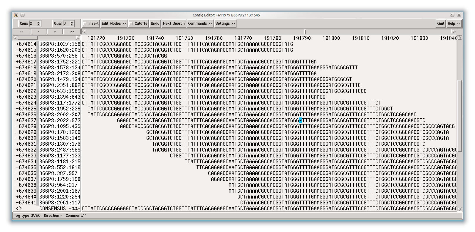 |
The "if you're lucky" part in the preceding sentence is not there by accident: having so many clean reads is more of an exception rather a rule. On the other hand, most sequencing errors in current IonTorrent data are unproblematic ... if it were not for indels, which is going to be explained on the next sections.
The main source of error in your data will be insertions / deletions (indels) especially in homopolymer regions (but not only there, see also next section). Starting with a base run of 4 to 6 bases, there is a distinct tendency to have an increased occurrence of indel errors.

The above figure contains a couple of particularly nasty indel problems. While areas 2 (C-homopolymer length 3), 5 (A-homopolymer length 4) and 6 (T-homopolymer length 3) are not a big problem as most of the reads got the length right, the areas 1, 3 and 4 are nasty.
Area 1 is an A-homopolymer of length 7 and while many reads get that length right (enough to tell MIRA what the true length is), it also contains reads with a length of 6 and and others with a length of 8.
Area 2 is a "A-homopolymer" of length 2 where approximately half of the reads get the length right, the other half not. See also the following section.
Area 4 is a T-homopolymer of length 5 which also has approximately half the reads with a wrong length of 4.
In the previous section, the screen shot showing indels had an indel at a homopolymer of 2, which is something quite curious. Upon closer investigation, one might notice a pattern in the gap/nogap distribution: it is almost identical to the orientation of build direction of reads!
I looked for other examples of this behaviour and found quite a number of them, the following figure shows a very clear case of that error behaviour:
Figure 11.10. Example for a sequencing direction dependent indel. Note how all but one of the reads in '+' direction miss a base while all reads built in in '-' direction have the correct number of bases.
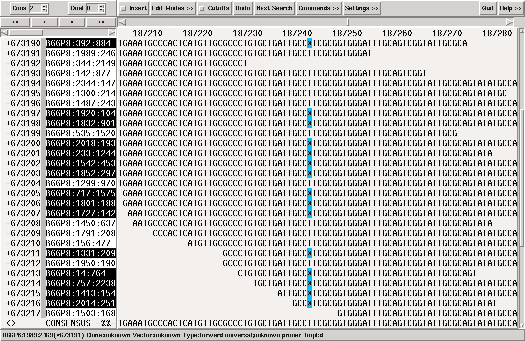 |
This is quite astonishing: the problem occurs at a site without real homopolymer (calling a 2-bases run a 'homopolymer' starts stretching the definition a bit) and there are no major problematic homopolymer sites near. In fact, this was more or less the case for all sites I had a look at.
Neither did the cases which were investigated show common base patterns, so unlike the Solexa GGCxG motif it does not look like that error of IonTorrent is bound to a particular motif.
While I cannot prove the following statement, I somehow suspect that
there must be some kind of secondary structure forming which leads to
that kind of sequencing error. If anyone has a good explanation I'd be
happy to hear it: feel free to contact me at
<bach@chevreux.org>.
The coverage variance with the old ~100bp reads was a bit on the bad side for low coverage projects (10x to 15x): it varied wildly, sometimes dropping to nearly zero, sometimes reaching approximately double the coverage.
This has now improved and I have not seen pronounced coverage variance in the data sets I have worked on.
The GC bias seems to be small to non-existent, at least I could not immediately make a correlation between GC content and coverage.
You will want to keep an eye on the clipping of the data in the SFF files from IonTorrent: while it is generally good enough, some data sets of IonTorrent show that - for some error patterns - the clipping is too lax and strange artefacts appear. MIRA will take care of these - or at least of those it knows - but you should be aware of this potential problem.
IonTorrent being pretty new, getting as much information on that technology is quite important. So here are a couple of links I found to be helpful:
There is, of course, the TorrentDev site (http://lifetech-it.hosted.jivesoftware.com/community/torrent_dev) at Life Technologies which will be helpful to get a couple of questions answered.
Just be aware that some of the documents over there are sometimes painting an - how should I say it diplomatically? - overly optimistic view on the performance of the technology. On the other hand, so do documents released by the main competitors like 454/Roche, Illumina, PacBio etc. ... so no harm done there.
I found Nick Loman's blog Pathogens: Genes and Genomes to be my currently most valuable source of information on IonTorrent. While the group he works for won a sequencer from IonTorrent, he makes that fact very clear and still unsparingly dissects the data he gets from that machine.
His posts got me going in getting MIRA grok IonTorrent.
The blog of Lex Nederbragt In between lines of code is playing in the same league: very down to earth and he knows a bluff when he sees it ... and is not afraid to call it (be it from IonTorrent, PacBio or 454).
The analysis he did on a couple of Ion data sets have saved me quite some time.
Last, but not least, the board with IonTorrent-related-stuff over at SeqAnswers, the first and foremost one-stop-shop ... erm ... discussion board for everything related to sequencing nowadays.
As of January 2014, PacBio should be seen as the technology to go to for de-novo sequencing of bacteria and lower eukaryotes. Period. Complement it with a bit of Illumina to get rid of the last remaining errors and you'll have - for a couple of thousand Euros - the best genome sequences money can buy.
Just one word: huge. At least compared to other currently existing technologies. It is not unusual to get average - usable - read lengths of more than 3 to 4 kb, some chemistries doubling that number (at the expense of accuracy). The largest - usable - reads I have seen were > 25kb, though one needs to keep in mind that these are quite rare and one does not see many of them in a project.
I have seen none in my projects so far, neither have I in public data. But these were certainly not as many projects as Sanger, 454, Illumina and Ion, so take this with a grain of salt.
Once the raw PacBio data has been corrected (HGAP pipeline), the resulting reads have a pretty good accuracy. There still are occasional homopolymer errors remaining at non-random locations, but they are a minor problem.
The assemblies coming out of the HGAP pipeline are already astoundingly good. Of course you get long contigs, but also the number of miscalled consensus bases is not too bad: 1 error per 20 kb. Once the program Quiver went through the assembly to do its magic in polishing, the quality improves further to into the range of 1 error per 50kb to 1 error per 250kb.
In my hands, I get even better assemblies with MIRA (longer contigs which span repeats unresolved by HGAP). When combining this with some low coverage Illumina data (say, 50x) to do cheap polishing, the error rates I get are lower than 1 error in 4 megabases.
| Note |
|---|---|
| Take the above with a grain of salt as at the time of this writing, I analysed in-depth only on a couple of bacteria. For ploidal organisms I have just played a bit around with public data without really doing an in depth analysis there. |
With PacBio, there are quite a number of read types being thrown around and which do confuse people: polymerase reads, quality clipped reads, subreads, corrected reads and maybe some more I currently forgot. Here's the total unofficial guide on how to keep those things apart:
polymerase reads are the rawest and most unedited stuff you may come into contact. You can see it as "data fresh from the machine" and the number of megabases there is usually the one sequencing providers sell to you.
The sequencing technology PacBio employs uses special hairpin adaptors they have named SMRTBell, and these adaptors will be present in the polymerase reads together with the fragments of your DNA.
In terms of regular expression look-alike, the data in polymerase reads has the following form:
(Adaptor + (forward fragment sequence + (Adaptor + (fragment sequence in reverse complement))))*
E.g., some of your polymerase reads will contain just the adaptor and (part of) a fragment sequence: Adap+FwdSeq. Others might contain: Adap+FwdSeq+Adap+RevSeq. And still others might contain: multiple copies of Adap+FwdSeq+Adap+RevSeq.
- quality clipped reads are simply polymerase reads where some sort of first quality clipping has been done.
- subreads are quality clipped reads where the adaptors have been removed and the read split into forward fragment sequences and reverse fragment sequences. Hence, one quality clipped polymerase read can yield several subreads.
corrected (sub)reads are subreads where through the magic of lots of computational power and a very high coverage of subreads, the errors have been almost completely removed from the subreads.
This is usually done only on a part of the subreads as it takes already long enough (several hundred hours CPU for a simple bacterium).
The splitting of polymerase reads into subreads (see above) needs the SMRTBell adaptor to be recognised by motif searching programs. Unfortunately, it looks like as if some "low percentage" of reads have a self-looped end instead of an adaptor. Which in turn means that the subread splitting will not split those reads and you end up with a chimeric sequence.
You need to be brave now: the accuracy of the the unclipped polymerase reads is usually only about 50%. That is: on average every second base is wrong. And I have seen a project where this accuracy was only 14% (6 out of 7 bases are wrong).
After clipping, the average accuracy of the polymerase reads should be anywhere between 80% and 85% (this depends a little bit on the chemistry used), which translates to: every 5th to every 7th base is wrong. The vast majority of errors being insertions or deletions, not base substitutions.
80% to 85% accurracy with indels as primary error is unfortunately something assemblers cannot use very well. Read: not at all if you want good assemblies (at least I know no program which does that). Therefore, one needs to apply some sort of correction ... which needs quite a deal of CPU, see below.
The above mentioned accuracies of 80% to 85% are too low for any existing assembler I know to be correctly assembled. Therefore, people came up with the idea of doing error correction on subreads to improve their quality.
There are two major approaches: 1) correcting PacBio subreads with other technologies with shorter reads and 2) correcting long PacBio subreads with shorter PacBio subreads. Both approaches have been shown to work, though there seems to be a preference nowadays to use the second option as the "shorter" PacBio reads provide the benefit of being still longer than read from other technologies and hence provide a better repeat resolution.
Anyway, the amount of CPU power needed for any method above is something to keep for: bacteria with 3 to 5 megabases at a 100x polymerase read coverage can take several hundred hours of CPU for the correction step.
This is a problem which cannot be really attributed to PacBio: one absolutely needs to check whether the protocols used "since ever" for DNA extraction yield results which are clean and long enough for PacBio. Often they are not.
The reason for this being a problem is simple: PacBio can sequence really long fragments, but if your DNA extraction protocol smashed the DNA into small pieces, then no sequencing technology in this universe will be able to give you long reads for small fragments.
Table of Contents
“ Reliable information lets you say 'I don't know' with real confidence. ” | ||
| --Solomon Short | ||
Well, duh! But it's interesting what kind of mails I sometimes get. Like in:
“We've sequenced a one gigabase, diploid eukaryote with Solexa 36bp paired-end with 200bp insert size at 25x coverage. Could you please tell us how to assemble this data set de-novo to get a finished genome?”
A situation like the above should have never happened. Good sequencing providers are interested in keeping customers long term and will therefore try to find out what exactly your needs are. These folks generally know their stuff (they're making a living out of it) and most of the time propose you a strategy that fulfills your needs for a near minimum amount of money.
Listen to them.
If you think they try to rip you off or are overselling their competences (which most providers I know won't even think of trying, but there are some), ask a quote from a couple of other providers. You'll see pretty quickly if there are some things not being right.
| Note |
|---|---|
| As a matter of fact, a rule which has saved me time and again for finding sequencing providers is not to go for the cheapest provider, especially if their price is far below quotes from other providers. They're cutting corners somewhere others don't cut for a reason. |
| Note |
|---|---|
| This is a slightly reworked version of a post I made on the MIRA talk mailing list. The question "Could you please recommend me a sequencing provider?" arrives every now and then in my private inbox, often enough for me decide to make a collage of the responses I gave in the past and post it to MIRA talk. |
This response got, errrr, a little longer, but allow me to note that I will not give you names. The reasons are manyfold:
- once upon a time I worked for a sequencing company
- the company I am currently employed with is not in the sequencing provider business, but the company uses more than one sequencing provider on a regular base and I get to see quite some data
- due to my development on MIRA in my free time, I'm getting insight into a number of highs and lows of sequencing technologies at different sequencing providers which I would not get if I were to expose them publicly ... I do not want to jeopardise these relationships.
That being said, there are a number of general considerations which could help you. Excuse me in case the detours I am going to make are obvious to you, but I'm writing this also for future references. Also, please bear with me if I look at "sequencing" a bit differently than you might be accustomed to from academia, but I have worked for quite some time now in industry ... and there cost-effectiveness respectively "probability of success" of a project as whole is paramount to everything else. I'll come back to that further down.
There's one -- and only one -- question which you, as sequencing customer, need to be able to answer ... if necessary in every excruciating detail, but you must know the answer. The question is:
The above makes it clear that, depending on what you are really interested in within your project and what you expect to be able to do with the sequencing data, one can cut corners and reduce cost here and there (but not everywhere). And therefore, the above question "What do you want?" is one which - after the initial chit-chat of "hi, hello, nice to meet you, a pleasure to be here, etc." - every good representative of respectable sequencing providers I have met so far will ask as very first question. Usually in the form of "what do you want to sequence and what will you want to use the data for (and what not)?"
... difference between "want" and "need" ...
Every other question - like where to sequence, which sequencing technology to use, how to process the sequencing data afterwards - is incidental and subordinated to your answer(s) to the question of "what do you want?!" But often sequencing customers get their priorities wrong by putting forward another question:
There's one last detour I'd like to make, and that is the question of "where to sequence?"
All of the above means that depending on what I need the data for, I have the freedom choose among different providers. In case I just need masses of raw data and potential savings are substantial, I might go with the cheapest whom I know to generate good data. If I want good service and second round of data in case I am not 110% satisfied with the first round (somehow people have stopped questioning me there), this is usually not the cheapest provider ... but the additional costs are not really high. If I wanted my data really really quick, I'd search for a provider with Ion Torrent, or MiSeq (I am actually looking for one with a MiSeq, so if anyone knows a good one, preferably in Europe -> mail me). Though I already did transcriptomics on eukaryotes, in case I needed larger eukaryotes assembled de-novo & also annotated, I would probably look for the help of a larger sequencing center as this starts to get dangerously near the fringe of my field of expertise.
In closing this part, here are a couple of guidelines which have not failed me so far for choosing sequencing providers:
- Building a good relationship helps. In case your institute / university already has good (or OK) experience with a provider, ask there first.
- It is a lot easier to build a good relationship with someone who speaks your language ... or a good(!) English.
- I will not haggle for a couple of hundred Euros in a single project, I'll certainly reconsider this when savings are in the tens of thousands.
- Managing expectations: some sequencing projects are high risk from the start, for lots of possible reasons (underfunded, bad starting material, unclear organism). This is *sometimes* (!) OK as long as everyone involved knows and acknowledges this. However, you should always have a clear target ("what am I looking for?") and preferably know in advance how to treat the data to get there.
- Errors occur, stay friendly at first. In case the expectations were clear (see above), the material and organism are not at fault but the data quality somehow is bad, it is not too difficult to have the sequencing provider acknowledge this and get additional sequencing for no added cost.
Regarding the technologies you can use ... it really depends on what you want to do :-) And note that I base my answers on technologies available today without bigger problems: PacBio, Illumina, with IonTorrent as Joker for quick projects. Since 2018, 454 can be considered to be dead as the Newbler assembler is not availöable anymore and I am not even sure sequencing kits are manufactured. Oxford Nanopore has become a game changer with reads of several hundred Kb and even over a megabase, but still requires quite some tinkering both in protocols and on the bioinformatics side.
Here's how I see things as of now (early 2019), which might not necessarily be how others see them.
Use for: checking assemblies; closing gaps by PCR; checking for a couple of genes with known sequence (i.e., where you can design oligos for).
Do not use for: anything else. In particular, if you find yourself designing oligos for a 96 well plate destined for Sanger sequencing of a single bacterial DNA sample, you (probably) are doing something wrong.
Use for: de-novo of bacteria and lower eukaryotes (or higher eukaryotes if you have the money). PacBio should be seen as the technology to use when getting the best good quality sequence with least number of contigs is important to you. Also, resequencing of variants of known organisms with lots of genomic reorganisation flexibility due to high numbers of transposons (where short reads will not help in getting the chromosome assembled/mapped correctly).
Do not use for: resequencing of "dull" organisms (where the only differences will be simple SNPs or simple insertion/deletions or simple contig reorganisations at non-repetitive places). Illumina will do a much better and cost effective job there.
| Note |
|---|---|
As of Fall 2018: aim for at least 100x coverage of raw data, better 130x to 150x as pre-processing (quality clip, removal of adapters and other sequencing artefacts) will take its toll and reduce the data by up to 1/3. After that, the error correction/self-correction of raw reads into corrected reads will again reduce the data considerably. It's really a numbers game: the more data you have, the more likely you will also get many of those really long reads in the 5 to 30 Kb range which are extremely useful to get over those nasty repeats. |
| Note |
|---|---|
| MIRA should not be used to assemble PacBio. Use it to polish the results of Canu or Falcon/Quiver/Arrow with Illumina data. |
| Warning |
|---|---|
| For non-haploid organisms, you might need more coverage to get enough data at ploidy sites to get the reads correctly out of error correction. Aim for at least 80x to 100x per ploidy. |
| Warning |
|---|---|
| Preparation of your DNA sample is not trivial as many methods will break your DNA into "small" chunks which are good enough for Sanger, 454, Illumina or Ion Torrents, but not for PacBio. |
I currently have no hands-on experience with ONT, but from what I see it gets you much longer reads than PacBio. At the moment I would go for it for de-novo of difficult eukaryotes or a quick and dirty first look bacteria with lots of repeats.
Use for: general resequencing jobs (finding SNPs, indel locations of any size, copy number variations etc.); gene expression analysis; cheap test sequencing of unknown organisms to assess complexity; de-novo sequencing if you are OK with getting hundreds / thousands of contigs (depending on organism, some bacteria get only a few dozen).
| Warning |
|---|---|
| Careful with high GC organisms, starting with 60% to 65% GC Illumina reads contain more errors: SNP detection may be less reliable if extreme care is not taken to perform good read clipping. Especially the dreaded GGCxG motif often leads to problems in Illumina reads. |
| Warning |
|---|---|
| For de-novo assemblies, do NOT (never ever at all and under no circumstances) use the Nextera kit, take TruSeq. The non-random fragmentation behaviour of Nextera leads to all sorts of problems for assemblers (not only MIRA) which try to use kmer frequencies as a criterion for repetitiveness of a given sequence. |
Use for: like Illumina. With three notable exceptions: 1) SNP detection is not as good as with Illumina (more false positives and false negatives) 2) de-novo assemblies will contain more single-base indels and 3) Ion having problems with homopolymers, that technology is not as well suited as complimentary hybrid technology for PacBio as is Illumina (except for high-GC perhaps).
Ion has a speed advantage on Illumina: if you have your own machine, getting from your sample to data takes less time than with Illumina.
Also, it looks like as if Ion has less problems with GC content or sequence motifs than Illumina.
- On a cheap gene fishing expedition? Probably Illumina HiSeq, at least 100bp, 150 to 250bp or 300bp if your provider supports it well. Paired-end definitely a plus. As alternative: Ion Torrent for small organism (maybe up to 100Mb) and when you need results quickly without caring for possible frameshifts.
- Want some larger contigs? PacBio. Add in cheap Illumina 100bp paired-end (150 to 300bp if provider supports it) to get rid of those last frameshifts which may remain.
- Even longer reads to resolve difficult areas? Some tinkering with Oxford Nanopore + polishing with Illumina should do wonders.
There is a reason why Illumina currently dominates the market as it does: a cheap Illumina run (preferably paired-end) will answer most of your questions in 95% of the cases. Things will get difficult for organisms with high numbers of repeats and/or frequent genome re-arrangements. Then using longer read technologies and/or Illumina mate-pair may be required.
There's one thing to be said about coverage and de-novo assembly: especially for bacteria, getting more than 'decent' coverage is cheap with any current day technology. Every assembler I know will be happy to assemble de-novo genomes with coverages of 25x, 30x, 40x ... and the number of contigs will still drop dramatically between a 15x Ion Torrent and a 30x Ion Torrent project.
In any case, do some calculations: if the coverage you expect to get reaches 50x (e.g. 200MB raw sequence for a 4MB genome), then you (respectively the assembler) can still throw away the worst 20% of the sequence (with lots of sequencing errors) and concentrate on the really, really good parts of the sequences to get you nice contigs.
Other example: the price for 1 gigabase Illumina paired-end of a single DNA prep is way, way below USD 1000, even with commercial providers. Then you just need to do the math: is it worth to invest 10, 20, 30 or more days of wet lab work, designing primers, doing PCR sequencing etc. and trying to close remaining gaps or hunt down sequencing errors when you went for a 'low' coverage or a non-hybrid sequencing strategy? Or do you invest a few bucks more to get some additional coverage and considerably reduce the uncertainties and gaps which remain?
Remember, you probably want to do research on your bug and not research on how to best assemble and close genomes. So even if you put (PhD) students on the job, it's costing you time and money if you wanted to save money earlier in the sequencing. Penny-wise and pound-foolish is almost never a good strategy :-)
I do agree that with eukaryotes, things start to get a bit more interesting from the financial point of view.
There is, however, a catch-22 situation with coverage: too much coverage isn't good either. Without going into details: sequencing errors sometimes interfere heavily when coverage exceeds ~60x to 80x for 454 & IonTorrent and approximately 150x to 200x for Solexa/Illumina.
In those cases, do yourself a favour: there's more than enough data for your project ... just cut it down to some reasonable amount: 40x to 50x for 454 & IonTorrent, 100x for Solexa/Illumina.
So, you have decided that sequencing your bug with PacBio and Illumina (or PacBio and Ion Torrent or whatever) may be a viable way to get the best bang for your buck. Then please follow this advice: prepare enough DNA in one go for the sequencing provider so that they can sequence it with all the technologies you chose without you having to prepare another batch ... or even grow another culture!
The reason for that is that as soon as you do that, the probability that there is a mutation somewhere that your first batch did not have is not negligible. And if there is a mutation, even if it is only one base, there is a >95% chance that MIRA will find it and thinks it is some repetitive sequence (like a duplicated gene with a mutation in it) and splits contigs at those places.
Now, there are times when you cannot completely be sure that different sequencing runs did not use slightly different batches (or even strains).
One example: the SFF files for SRA000156 and SRA001028 from the NCBI short trace archive should both contain E.coli K12 MG-16650 (two unpaired half plates and a paired-end plate). However, they contain DNA from different cultures. Furthermore, the DNA was prepared by different labs. The net effect is that the sequences in the paired-end library contain a few distinct mutations from the sequences in the two unpaired half-plates. Furthermore, the paired-end sequences contain sequences from phages that are not present in the unpaired sequences.
In those cases, provide strain information to the reads so that MIRA can discern possible repeats from possible SNPs.
The reason is simple: some bacteria grow so fast that they start replicating themselves even before having finished the first replication cycle. This leads to more DNA around the origin of replication being present in cells, which in turn fools assemblers and mappers into believing that those areas are either repeats or that there are copy number changes.
Sample. In. Stationary. Phase!
For de-novo assemblies, MIRA will warn you if it detects data which points at exponential phase. In mapping assemblies, look at the coverage profile of your genome: if you see a smile shape (or V shape), you have a problem.
This is a source of interesting problems and furthermore gets people wondering why MIRA sometimes creates more contigs than other assemblers when it usually creates less.
Here's the short story: there are data sets which include one ore several high-copy plasmid(s). Here's a particularly ugly example: SRA001028 from the NCBI short read archive which contains a plate of paired-end reads for Ecoli K12 MG1655-G (ftp://ftp.ncbi.nih.gov/pub/TraceDB/ShortRead/SRA001028/).
The genome is sequenced at ~10x coverage, but during the assembly, three intermediate contigs with ~2kb attain a silly maximum coverage of ~1800x each. This means that there were ~540 copies of this plasmid (or these plasmids) in the sequencing.
When using the uniform read distribution algorithm - which is switched on by default when using "--job=" and the quality level of 'accurate' - MIRA will find out about the average coverage of the genome to be at ~10x. Subsequently this leads MIRA to dutifully create ~500 additional contigs (plus a number of contig debris) with various incarnations of that plasmid at an average of ~10x, because it thought that these were repetitive sites within the genome that needed to be disentangled.
Things get even more interesting when some of the plasmid / phage copies are slightly different from each other. These too will be split apart and when looking through the results later on and trying to join the copies back into one contig, one will see that this should not be done because there are real differences.
DON'T PANIC!
The only effect this has on your assembly is that the number of contigs goes up. This in turn leads to a number of questions in my mailbox why MIRA is sometimes producing more contigs than Newbler (or other assemblers), but that is another story (hint: Newbler either collapses repeats or leaves them completely out of the picture by not assembling repetitive reads).
What you can do is the following:
either you assemble everything together and the join the plasmid contigs manually after assembly, e.g. in gap4 (drawback: on really high copy numbers, MIRA will work quite a bit longer ... and you will have a lot of fun joining the contigs afterwards)
or, after you found out about the plasmid(s) and know the sequence, you filter out reads in the input data which contain this sequence (you can use mirabait for this) and assemble the remaining reads.
Table of Contents
“Just when you think it's finally settled, it isn't. ” | ||
| --Solomon Short | ||
| Warning |
|---|---|
The documentation of MIRA 3.9.x has not completely caught up yet with the changes introduced by MIRA now using manifest files. Quite a number of recipes still show the old command-line style, e.g.: mira --project=... --job=... ... For those cases, please refer to chapter 3 (the reference) for how to write manifest files. |
If your sequencing provider gave you data which was NOT pre-clipped for vector sequence, you can do this yourself in a pretty robust manner using SSAHA2 -- or the successor, SMALT -- from the Sanger Centre. You just need to know which sequencing vector the provider used and have its sequence in FASTA format (ask your provider).
| Note |
|---|---|
| This screening is a valid method for any type of Sanger sequencing vectors, 454 adaptors, Illumina adaptors and paired-end adaptors etc. However, you probably want to use it only for Sanger type data as MIRA already knows all standard 454, Ion Torrent and Illumina adaptors. |
| Note |
|---|---|
| SSAHA2 and SMALT need their input data to be in FASTA format, so for these to run you will need them also in FASTA format. For MIRA however you can load your original data in whatever format it was present. |
For SSAHA2 follow these steps (most are the same as in the example above):
$ssaha2 -output ssaha2 -kmer 8 -skip 1 -seeds 1 -score 12 -cmatch 9 -ckmer 6 /path/where/the/vector/data/resides/vector.fastayourinputsequences.fasta>screendataforyoursequences.ssaha2
Then, in your manifest file, add the following line in the readgroup which contains the sequences you screened:
readgroup
...
data = yourinputsequences_inwhateverformat_thisexamplehasfastq.fastq
data = screendataforyoursequences.ssaha2
...
For SMALT, the only difference is that you use SMALT for generating the vector-screen file and ask SMALT to generate it in SSAHA2 format. As SMALT works in two steps (indexing and then mapping), you also need to perform it in two steps and then call MIRA. E.g.:
$smalt index -k 7 -s 1 smaltidxdb /path/where/the/vector/data/resides/vector.fasta$smalt map -f ssaha -d -1 -m 7 smaltidxdbyourinputsequences.fasta>screendataforyoursequences.smalt
| Note |
|---|---|
Please note that, due to subtle differences between output of SSAHA2 (in
ssaha2 format) and SMALT (in ssaha2 format), MIRA identifies the source
of the screening (and the parsing method it needs) by the name of the
screen file. Therefore, screens done with SSAHA2 need to have the
postfix .ssaha2 in the file name and screens done
with SMALT need
*.smalt.
|
Table of Contents
- 14.1. Assembly quality
- 14.2. 454 data
- 14.2.1. What do I need SFFs for?
- 14.2.2. What's sff_extract and where do I get it?
- 14.2.3. Do I need the sfftools from the Roche software package?
- 14.2.4. Combining SFFs
- 14.2.5. Adaptors and paired-end linker sequences
- 14.2.6. What do I get in paired-end sequencing?
- 14.2.7. Sequencing protocol
- 14.2.8. Filtering sequences by length and re-assembly
- 14.3. Solexa / Illumina data
- 14.4. Hybrid assemblies
- 14.5. Masking
- 14.6. Miscellaneous
- 14.7. Platforms and Compiling
“Every question defines its own answer. Except perhaps 'Why a duck?' ” | ||
| --Solomon Short | ||
| Warning |
|---|---|
The documentation of MIRA 3.9.x has not completely caught up yet with the changes introduced by MIRA now using manifest files. Quite a number of recipes still show the old command-line style, e.g.: mira --project=... --job=... ... For those cases, please refer to chapter 3 (the reference) for how to write manifest files. |
This list is a collection of frequently asked questions and answers regarding different aspects of the MIRA assembler.
| Note |
|---|---|
| This document needs to be overhauled. |
- 14.1.1. Test question 1
- 14.1.2. Test question 2
14.1.1. | Test question 1 |
Test answer 1 | |
14.1.2. | Test question 2 |
Test answer 2 |
	I have a project which I once started quite normally via
	"--job=denovo,genome,accurate,454"
	and once with explicitly switching off the uniform read distribution
	"--job=denovo,genome,accurate,454 -AS:urd=no"
	I get less contigs in the second case and I wonder if that is not better.
	Can you please explain?
Since 2.9.24x1, MIRA has a feature called "uniform read distribution" which is normally switched on. This feature reduces over-compression of repeats during the contig building phase and makes sure that, e.g., a rRNA stretch which is present 10 times in a bacterium will also be present approximately 10 times in your result files.
It works a bit like this: under the assumption that reads in a project are uniformly distributed across the genome, MIRA will enforce an average coverage and temporarily reject reads from a contig when this average coverage multiplied by a safety factor is reached at a given site.
It's generally a very useful tool disentangle repeats, but has some slight secondary effects: rejection of otherwise perfectly good reads. The assumption of read distribution uniformity is the big problem we have here: of course it's not really valid. You sometimes have less, and sometimes more than "the average" coverage. Furthermore, the new sequencing technologies - 454 perhaps but especially the microreads from Solexa & probably also SOLiD - show that you also have a skew towards the site of replication origin.
One example: let's assume the average coverage of your project is 8 and by chance at one place you have 17 (non-repetitive) reads, then the following happens:
$p$= parameter of -AS:urdsip
Pass 1 to $p-1$: MIRA happily assembles everything together and calculates a number of different things, amongst them an average coverage of ~8. At the end of pass '$p-1$', it will announce this average coverage as first estimate to the assembly process.
Pass $p$: MIRA has still assembled everything together, but at the end of each pass the contig self-checking algorithms now include an "average coverage check". They'll invariably find the 17 reads stacked and decide (looking at the -AS:urdct parameter which I now assume to be 2) that 17 is larger than 2*8 and that this very well may be a repeat. The reads get flagged as possible repeats.
Pass $p+1$ to end: the "possibly repetitive" reads get a much tougher treatment in MIRA. Amongst other things, when building the contig, the contig now looks that "possibly repetitive" reads do not over-stack by an average coverage multiplied by a safety value (-AS:urdcm) which I'll assume in this example to be 1.5. So, at a certain point, say when read 14 or 15 of that possible repeat want to be aligned to the contig at this given place, the contig will just flatly refuse and tell the assembler to please find another place for them, be it in this contig that is built or any other that will follow. Of course, if the assembler cannot comply, the reads 14 to 17 will end up as contiglet (contig debris, if you want) or if it was only one read that got rejected like this, it will end up as singlet or in the debris file.
Tough luck. I do have ideas on how to re-integrate those reads at the and of an assembly, but I had deferred doing this as in every case I had looked up, adding those reads to the contigs wouldn't have changed anything ... there's already enough coverage. What I do in those cases is simply filter away the contiglets (defined as being of small size and having an average coverage below the average coverage of the project / 3 (or 2.5)) from a project.
	When using uniform read distribution there are too many contig with low
	coverage which I don't want to integrate by hand in the finishing process. How
	do I filter for "good" contigs?
OK, let's get rid of the cruft. It's easy, really: you just need to look up one number, take two decisions and then launch a command.
The first decision you need to take is on the minimum average coverage the
contigs you want to keep should have. Have a look at the file
*_info_assembly.txt which is in the info directory after
assembly. In the "Large contigs" section, there's a "Coverage assessment"
subsection. It looks a bit like this:
	...
	Coverage assessment:
	--------------------
	Max coverage (total): 43
	Max coverage
	Sanger: 0
	454:    43
	Solexa: 0
	Solid:  0
	Avg. total coverage (size ≥ 5000): 22.30
	Avg. coverage (contig size ≥ 5000)
	Sanger: 0.00
	454:    22.05
	Solexa: 0.00
	Solid:  0.00
	...
This project was obviously a 454 only project, and the average coverage for it is ~22. This number was estimated by MIRA by taking only contigs of at least 5Kb into account, which for sure left out everything which could be categorised as debris. It's a pretty solid number.
Now, depending on how much time you want to invest performing some manual polishing, you should extract contigs which have at least the following fraction of the average coverage:
2/3 if a quick and "good enough" is what you want and you don't want to do some manual polishing. In this example, that would be around 14 or 15.
1/2 if you want to have a "quick look" and eventually perform some contig joins. In this example the number would be 11.
1/3 if you want quite accurate and for sure not loose any possible repeat. That would be 7 or 8 in this example.
The second decision you need to take is on the minimum length your contigs should have. This decision is a bit dependent on the sequencing technology you used (the read length). The following are some rules of thumb:
Sanger: 1000 to 2000
454 GS20: 500
454 FLX: 1000
454 Titanium: 1500
Let's assume we decide for an average coverage of 11 and a minimum length of 1000 bases. Now you can filter your project with miraconvert
miraconvert -x 1000 -y 11 sourcefile.caf filtered.caf
	I would like to find those places where MIRA wasn't sure and give it a quick
	shot. Where do I need to search?
Search for the following tags in gap4 or any other finishing program for finding places of importance (in this order).
IUPc
UNSc
SRMc
WRMc
STMU (only hybrid assemblies)
STMS (only hybrid assemblies)
- 14.2.1. What are little boys made of?
- 14.2.2. What are little girls made of?
14.2.1. | What are little boys made of? |
Snips and snails and puppy dog tails. | |
14.2.2. | What are little girls made of? |
Sugar and spice and everything nice. |
I need the .sff files for MIRA to load ...
Nope, you don't, but it's a common misconception. MIRA does not load SFF files, it loads FASTA, FASTA qualities, FASTQ, XML, CAF, EXP and PHD. The reason why one should start from the SFF is: those files can be used to create a XML file in TRACEINFO format. This XML contains the absolutely vital information regarding clipping information of the 454 adaptors (the sequencing vector of 454, if you want).
For 454 projects, MIRA will then load the FASTA, FASTA quality and the corresponding XML. Or from CAF, if you have your data in CAF format.
How do I extract the sequence, quality and other values from SFFs?
Use the sff_extract script from Jose Blanca at the University of Valencia to extract everything you need from the SFF files (sequence, qualities and ancillary information). The home of sff_extract is: http://bioinf.comav.upv.es/sff_extract/index.html but I am thankful to Jose for giving permission to distribute the script in the MIRA 3rd party package (separate download).
No, not anymore. Use the sff_extract script to extract your reads. Though the Roche sfftools package contains a few additional utilities which could be useful.
	I am trying to use MIRA to assemble reads obtained with the 454 technology
	but I can't combine my sff files since I have two files obtained with GS20
	system and 2 others obtained with the GS-FLX system. Since they use
	different cycles (42 and 100) I can't use the sfffile to combine both.
You do not need to combine SFFs before translating them into something MIRA (or other software tools) understands. Use sff_extract which extracts data from the SFF files and combines this into input files.
	I have no idea about the adaptor and the linker sequences, could you send me
	the sequences please?
Here are the sequences as filed by 454 in their patent application:
	>AdaptorA
	CTGAGACAGGGAGGGAACAGATGGGACACGCAGGGATGAGATGG
	>AdaptorB
	CTGAGACACGCAACAGGGGATAGGCAAGGCACACAGGGGATAGG
However, looking through some earlier project data I had, I also retrieved the following (by simply making a consensus of sequences that did not match the target genome anymore):
	>5prime454adaptor???
	GCCTCCCTCGCGCCATCAGATCGTAGGCACCTGAAA
	>3prime454adaptor???
	GCCTTGCCAGCCCGCTCAGATTGATGGTGCCTACAG
Go figure, I have absolutely no idea where these come from as they also do not comply to the "tcag" ending the adaptors should have.
I currently know one linker sequence (454/Roche also calls it spacer for GS20 and FLX paired-end sequencing:
	>flxlinker
	GTTGGAACCGAAAGGGTTTGAATTCAAACCCTTTCGGTTCCAAC
For Titanium data using standard Roche protocol, you need to screen for two linker sequences:
	>titlinker1
	TCGTATAACTTCGTATAATGTATGCTATACGAAGTTATTACG
	>titlinker2
	CGTAATAACTTCGTATAGCATACATTATACGAAGTTATACGA
| Warning |
|---|---|
| Some sequencing labs modify the adaptor sequences for tagging and similar things. Ask your sequencing provider for the exact adaptor and/or linker sequences. |
	Another question I have is does the read pair sequences have further
	adaptors/vectors in the forward and reverse strands?
Like for normal 454 reads - the normal A and B adaptors can be present in paired-end reads. That theory this could could look like this:
A-Adaptor - DNA1 - Linker - DNA2 - B-Adaptor.
It's possible that one of the two DNA fragments is *very* short or is missing completely, then one has something like this:
A-Adaptor - DNA1 - Linker - B-Adaptor
or
A-Adaptor - Linker - DNA2 - B-Adaptor
And then there are all intermediate possibilities with the read not having one of the two adaptors (or both). Though it appears that the majority of reads will contain the following:
DNA1 - Linker - DNA2
There is one caveat: according to current paired-end protocols, the sequences will NOT have the direction
---> Linker <---
as one might expect when being used to Sanger Sequencing, but rather in this direction
<--- Linker --->
Is there a way I can find out which protocol was used?
Yes. The best thing to do is obviously to ask your sequencing provider.
If this is - for whatever reason - not possible, this list might help.
Are the sequences ~100-110 bases long? It's GS20.
Are the sequences ~220-250 bases long? It's FLX.
Are the sequences ~350-450 bases long? It's Titanium.
Do the sequences contain a linker (GTTGGAACCGAAAGGGTTTGAATTCAAACCCTTTCGGTTCCAAC)? It's a paired end protocol.
If the sequences left and right of the linker are ~29bp, it's the old short paired end (SPET, also it's most probably from a GS20). If longer, it's long paired-end (LPET, from a FLX).
I have two datasets of ~500K sequences each and the sequencing company
already did an assembly (using MIRA) on the basecalled and fully processed
reads (using of course the accompanying *qual file). Do you suggest that I
should redo the assembly after filtering out sequences being shorter than a
certain length (e.g. those that are <200bp)? In other words, am I taking into
account low quality sequences if I do the assembly the way the sequencing
company did it (fully processed reads + quality files)?
I don't think that filtering out "shorter" reads will bring much positive improvement. If the sequencing company used the standard Roche/454 pipeline, the cut-offs for quality are already quite good, remaining sequences should be, even when being < 200bp, not of bad quality, simply a bit shorter.
Worse, you might even introduce a bias when filtering out short sequences: chemistry and library construction being what they are (rather imprecise and sometimes problematic), some parts of DNA/RNA yield smaller sequences per se ... and filtering those out might not be the best move.
You might consider doing an assembly if the company used a rather old version of MIRA (<3.0.0 for sure, perhaps also <3.0.5).
	Suppose you ran the genome of a strain that had one or more large
	deletions. Would it be clear from the data that a deletion had occurred?
In the question above, I assume you'd compare your strain X to a strain Ref and that X had deletions compared to Ref. Furthermore, I base my answer on data sets I have seen, which presently were 36 and 76 mers, paired and unpaired.
Yes, this would be clear. And it's a piece of cake with MIRA.
Short deletions (1 to 10 bases): they'll be tagged SROc or WRMc. General rule: deletions of up to 10 to 12% of the length of your read should be found and tagged without problem by MIRA, above that it may or may not, depending a bit on coverage, indel distribution and luck.
Long deletions (longer than read length): they'll be tagged with MCVc tag by MIRA ins the consensus. Additionally, when looking at the FASTA files when running the CAF result through miraconvert: long stretches of sequences without coverage (the @ sign in the FASTAs) of X show missing genomic DNA.
	Suppose you ran the genome of a strain X that had a plasmid missing from the
	reference sequence. Alternatively, suppose you ran a strain that had picked
	up a prophage or mobile element lacking in the reference. Would that
	situation be clear from the data?
Short insertions (1 to 10 bases): they'll be tagged SROc or WRMc. General rule: deletions of up to 10 to 12% of the length of your read should be found and tagged without problem by MIRA, above that it may or may not, depending a bit on coverage, indel distribution and luck.
Long insertions: it's a bit more work than for deletions. But if you ran a de-novo assembly on all reads not mapped against your reference sequence, chances are good you'd get good chunks of the additional DNA put together
Once the Solexa paired-end protocol is completely rolled out and used on a regular base, you would even be able to place the additional element into the genome (approximately).
	Any chance you could assemble de-novo the sequence of a from just the Solexa
	data?
| Warning |
|---|---|
| Highly opinionated answer ahead, your mileage may vary. |
Allow me to make a clear statement on this: maybe.
But the result would probably be nothing I would call a good assembly. If you used anything below 76mers, I'm highly sceptical towards the idea of de-novo assembly with Solexa (or ABI SOLiD) reads that are in the 30 to 50bp range. They're really too short for that, even paired end won't help you much (especially if you have library sizes of just 200 or 500bp). Yes, there are papers describing different draft assemblers (SHARCGS, EDENA, Velvet, Euler and others), but at the moment the results are less than thrilling to me.
If a sequencing provider came to me with N50 numbers for an assembled genome in the 5-8 Kb range, I'd laugh him in the face. Or weep. I wouldn't dare to call this even 'draft'. I'd just call it junk.
On the other hand, this could be enough for some purposes like, e.g., getting a quick overview on the genetic baggage of a bug. Just don't expect a finished genome.
Hybrid assemblies are assemblies where one used more than one sequencing technology. E.g.: Sanger and 454, or 454 and Solexa, or Sanger and Solexa etc.pp
Basically, one can choose two routes: multi-step or all-in-one-go.
Multi-steps means: to assemble reads from one sequencing technology (ideally the one from the shorter tech like, e.g., Solexa), fragment the resulting contigs into pseudo-reads of the longer tech and assemble these with the real reads from the longer tech (like, e.g., 454). The advantage of this approach is that it will be probably quite faster than the all-in-one-go approach. The disadvantage is that you loose a lot of information when using only consensus sequence of the shorter read technology for the final assembly.
All-in-one-go means: use all reads in one single assembly. The advantage of this is that the resulting alignment will be made of true reads with a maximum of information contained to allow a really good finishing. The disadvantage is that the assembly will take longer and will need more RAM.
	In EST projects, do you think that the highly repetitive option will get rid
	of the repetitive sequences without going to the step of repeat masking?
For eukaryotes, yes. Please also consult the [-KS:mnr] option.
Remember: you still MUST have sequencing vectors and adaptors clipped! In EST sequences the poly-A tails should be also clipped (or let mira do it.
For prokaryotes, I´m a big fan of having a first look at unmasked data. Just try to start MIRA without masking the data. After something like 30 minutes, the all-vs-all comparison algorithm should be through with a first comparison round. grep the log for the term "megahub" ... if it doesn't appear, you probably don't need to mask repeats
I want to mask away some sequences in my input. How do I do that?
First, if you want to have Sanger sequencing vectors (or 454 adaptor sequences) "masked", please note that you should rather use ancillary data files (CAF, XML or EXP) and use the sequencing or quality clip options there.
Second, please make sure you have read and understood the documentation for all -CL parameters in the main manual, but especially -CL:mbc:mbcgs:mbcmfg:mbcmeg as you might want to switch it on or off or set different values depending on your pipeline and on your sequencing technology.
You can without problem mix your normal repeat masking pipeline with the FASTA or EXP input for MIRA, as long as you mask and not clip the sequence.
An example:
	>E09238ARF0
	tcag GTGTCAGTGTTGACTGTAAAAAAAAAGTACGTATGGACTGCATGTGCATGTCATGGTACGTGTCA
	GTCAGTACAAAAAAAAAAAAAAAAAAAAGTACGT tgctgacgcacatgatcgtagc
(spaces inserted just as visual helper in the example sequence, they would not occur in the real stuff)
The XML will contain the following clippings: left clip = 4 (clipping away the "tcag" which are the last four bases of the adaptor used by Roche) right clip= ~90 (clipping away the "tgctgac..." lower case sequence on the right side of the sequence above.
Now, on the FASTA file that was generated with reads_sff.py or with the Roche sff* tools, you can let run, e.g., a repeat masker. The result could look like this:
	>E09238ARF0
	tcag XXXXXXXXX TTGACTGTAAAAAAAAAGTACGTATGGACTGCATGTGCATGTCATGGTACGTGTCA
	GTCAGTACAAAAAAAAAAAAAAAAAAAAGTACGT tgctgacgcacatgatcgtagc
The part with the Xs was masked away by your repeat masker. Now, when MIRA loads the FASTA, it will first apply the clippings from the XML file (they're still the same). Then, if the option to clip away masked areas of a read (-CL:mbc, which is normally on for EST projects), it will search for the stretches of X and internally also put clips to the sequence. In the example above, only the following sequence would remain as "working sequence" (the clipped parts would still be present, but not used for any computation.
	>E09238ARF0
	...............TTGACTGTAAAAAAAAAGTACGTATGGACTGCATGTGCATGTCATGGTACGTGTCA
	GTCAGTACAAAAAAAAAAAAAAAAAAAAGTACGT........................
Here you can also see the reason why your filters should mask and not clip the sequence. If you change the length of the sequence, the clips in the XML would not be correct anymore, wrong clippings would be made, wrong sequence reconstructed, chaos ensues and the world would ultimately end. Or something.
IMPORTANT! It might be that you do not want MIRA to merge the masked part of your sequence with a left or right clip, but that you want to keep it something like DNA - masked part - DNA. In this case, consult the manual for the -CL:mbc switch, either switch it off or set adequate options for the boundaries and gap sizes.
Now, if you look at the sequence above, you will see two possible poly-A tails ... at least the real poly-A tail should be masked else you will get megahubs with all the other reads having the poly-A tail.
You have two possibilities: you mask yourself with an own program or you let MIRA do the job (-CL:cpat, which should normally be on for EST projects but I forgot to set the correct switch in the versions prior to 2.9.26x3, so you need to set it manually for 454 EST projects there).
IMPORTANT! Never ever at all use two poly-A tail masker (an own and the one from MIRA): you would risk to mask too much. Example: assume the above read you masked with a poly-A masker. The result would very probably look like this:
	>E09238ARF0
	tcag XXXXXXXXX TTGACTGTAAAAAAAAAGTACGTATGGACTGCATGTGCATGTCATGGTACGTGTCA
	GTCAGTAC XXXXXXXXXXXXXXXXXXXX GTACGT tgctgacgcacatgatcgtagc
And MIRA would internally make the following out of it after loading:
	>E09238ARF0
	...............TTGACTGTAAAAAAAAAGTACGTATGGACTGCATGTGCATGTCATGGTACGTGTCA
	GTCAGTAC..................................................
and then apply the internal poly-A tail masker:
	>E09238ARF0
	...............TTGACTGT................................................
	..........................................................
You'd be left with ... well, a fragment of your sequence.
	I looked in the log file and that term "megahub" you told me about appears
	pretty much everywhere. First of all, what does it mean?
Megahub is the internal term for MIRA that the read is massively repetitive with respect to the other reads of the projects, i.e., a read that is a megahub connects to an insane number of other reads.
This is a clear sign that something is wrong. Or that you have a quite repetitive eukaryote. But most of the time it's sequencing vectors (Sanger), A and B adaptors or paired-end linkers (454), unmasked poly-A signals (EST) or non-normalised EST libraries which contain high amounts of housekeeping genes (always the same or nearly the same).
Countermeasures to take are:
set clips for the sequencing vectors (Sanger) or Adaptors (454) either in the XML or EXP files
for ESTs, mask poly-A in your input data (or let MIRA do it with the -CL:cpat parameter)
only after the above steps have been made, use the [-KS:mnr] switch to let mira automatically mask nasty repeats, adjust the threshold with [-SK:rt].
if everything else fails, filter out or mask sequences yourself in the input data that come from housekeeping genes or nasty repeats.
	While processing some contigs with repeats i get
	"Accepting probably misassembled contig because of too many iterations."
	What is this?
That's quite normal in the first few passes of an assembly. During each pass (-AS:nop), contigs get built one by one. After a contig has been finished, it checks itself whether it can find misassemblies due to repeats (and marks these internally). If no misassembly, perfect, build next contig. But if yes, the contig requests immediate re-assembly of itself.
But this can happen only a limited number of times (governed by -AS:rbl). If there are still misassemblies, the contig is stored away anyway ... chances are good that in the next full pass of the assembler, enough knowledge has been gained top correctly place the reads.
So, you need to worry only if these messages still appear during the last pass. The positions that cause this are marked with "SRMc" tags in the assemblies (CAF, ACE in the result dir; and some files in the info dir).
What are the debris composed of?
sequences too short (after trimming)
megahubs
sequences almost completely masked by the nasty repeat masker ([-KS:mnr])
singlets, i.e., reads that after an assembly pass did not align into any contig (or where rejected from every contig).
sequences that form a contig with less reads than defined by [-AS:mrpc]
I do not understand why ... happened. Is there a way to find out?
Yes. The tmp directory contains, beside temporary data, a number of log files with more or less readable information. While development versions of MIRA keep this directory after finishing, production versions normally delete this directory after an assembly. To keep the logs and temporary file also in production versions, use "-OUT:rtd=no".
As MIRA also tries to save as much disk space as possible, some logs and temporary files are rotated (which means that old logs and tmps get deleted). To switch off this behaviour, use "-OUT:rrot=no". Beware, the size of the tmp directory will increase, sometimes dramatically so.
How MIRA clipped the reads after loading them can be found in the file
mira_int_clippings.0.txt. The entries look like this:
load: minleft. U13a01d05.t1 Left: 11 -> 30
Interpret this as: after loading, the read "U13a01d05.t1" had a left clipping of eleven. The "minleft" clipping option of MIRA did not like it and set it to 30.
load: bad seq. gnl|ti|1133527649 Shortened by 89 New right: 484
Interpret this as: after loading, the read "gnl|ti|1133527649" was checked with the "bad sequence search" clipping algorithm which determined that there apparently is something dubious, so it shortened the read by 89 bases, setting the new right clip to position 484.
Also, is MIRA be available on a windows platform?
As a matter of fact: it was and may be again. While I haven't done it myself, according to reports I got compiling MIRA 2.9.3* in a Cygwin environment was actually painless. But since then BOOST and multi-threading has been included and I am not sure whether it is still as easy.
I'd be thankful for reports :-)
Table of Contents
“Design flaws travel in herds. ” | ||
| --Solomon Short | ||
| Warning |
|---|---|
The documentation of MIRA 3.9.x has not completely caught up yet with the changes introduced by MIRA now using manifest files. Quite a number of recipes still show the old command-line style, e.g.: mira --project=... --job=... ... For those cases, please refer to chapter 3 (the reference) for how to write manifest files. |
This documents describes purpose and format of the MAF format, version 1. Which has been superceeded by version 2 but is not described here (yet). But as v1 and v2 are very similar only the notion of readgroups is a big change, I'll let this description live until I have time to update this section.
I had been on the hunt for some time for a file format that allow MIRA to quickly save and load reads and full assemblies. There are currently a number of alignment format files on the market and MIRA can read and/or write most of them. Why not take one of these? It turned out that all (well, the ones I know: ACE, BAF, CAF, CALF, EXP, FRG) have some kind of no-go 'feature' (or problem or bug) that makes one life pretty difficult if one wants to write or parse that given file format.
What I needed for MIRA was a format that:
is easy to parse
is quick to parse
contains all needed information of an assembly that MIRA and many finishing programs use: reads (with sequence and qualities) and contigs, tags etc.pp
MAF is not a format with the smallest possible footprint though it fares quite well in comparison to ACE, CAF and EXP), but as it's meant as interchange format, it'll do. It can be easily indexed and does not need string lookups during parsing.
I took the liberty to combine many good ideas from EXP, BAF, CAF and FASTQ while defining the format and if anything is badly designed, it's all my fault.
This describes version 1 of the MAF format. If the need arises, enhancements like meta-data about total number of contigs and reads will be implemented in the next version.
MAF ...
... has for each record a keyword at the beginning of the line, followed by exactly one blank (a space or a tab), then followed by the values for this record. At the moment keywords are two character keywords, but keywords with other lengths might appear in the future
... is strictly line oriented. Each record is terminated by a newline, no record spans across lines.
All coordinates start at 1, i.e., there is no 0 value for coordinates.
Here's an example for a simple read, just the read name and the sequence:
	  RD      U13a05e07.t1
	  RS      CTTGCATGCCTGCAGGTCGACTCTAGAAGGACCCCGATCA
	  ER
Reads start with RD and end with ER, the RD keyword is always followed by the name of the read, ER stands on its own. Reads also should contain a sequence (RS). Everything else is optional. In the following example, the read has additional quality values (RQ), template definitions (name in TN, minimum and maximum insert size in TF and TT), a pointer to the file with the raw data (SF), a left clip which covers sequencing vector or adaptor sequence (SL), a left clip covering low quality (QL), a right clip covering low quality (QR), a right clip covering sequencing vector or adaptor sequence (SR), alignment to original sequence (AO), a tag (RT) and the sequencing technology it was generated with (ST).
	  RD      U13a05e07.t1
	  RS      CTTGCATGCCTGCAGGTCGACTCTAGAAGGACCCCGATCA
	  RQ      ,-+*,1-+/,36;:6≤3327<7A1/,,).('..7=@E8:
	  TN      U13a05e07
	  DI      F
	  TF      1200
	  TT      1800
	  SF      U13a05e07.t1.scf
	  SL      4
	  QL      7
	  QR      30
	  SR      32
	  AO      1 40 1 40
	  RT      ALUS 10 15 Some comment to this read tag.
	  ST      Sanger
	  ER
RD string: readname
RD followed by the read name starts a read.
LR integer: read length
The length of the read can be given optionally in LR. This is meant to help the parser perform sanity checks and eventually pre-allocate memory for sequence and quality.
MIRA at the moment only writes LR lines for reads with more than 2000 bases.
RS string: DNA sequence
Sequence of a read is stored in RS.
RQ string: qualities
Qualities are stored in FASTQ format, i.e., each quality value + 33 is written as single as ASCII character.
SV string: sequencing vector
Name of the sequencing vector or adaptor used in this read.
TN string: template name
Template name. This defines the DNA template a sequence comes from. In it's simplest form, a DNA template is sequenced only once. In paired-end sequencing, a DNA template is sequenced once in forward and once in reverse direction (Sanger, 454, Solexa). In Sanger sequencing, several forward and/or reverse reads can be sequenced from a DNA template. In PacBio sequencing, a DNA template can be sequenced in several "strobes", leading to multiple reads on a DNA template.
DI character: F or R
Direction of the read with respect to the template. F for forward, R for reverse.
TF integer: template size from
Minimum estimated size of a sequencing template. In paired-end sequencing, this is the minimum distance of the read pair.
TT integer: template size to
Maximum estimated size of a sequencing template. In paired-end sequencing, this is the maximum distance of the read pair.
SF string: sequencing file
Name of the sequencing file which contains raw data for this read.
SL integer: seqvec left
Clip left due to sequencing vector. Assumed to be 1 if not present. Note that left clip values are excluding, e.g.: a value of '7' clips off the left 6 bases.
QL integer: qual left
Clip left due to low quality. Assumed to be 1 if not present. Note that left clip values are excluding, e.g.: a value off '7' clips of the left 6 bases.
CL integer: clip left
Clip left (any reason). Assumed to be 1 if not present. Note that left clip values are excluding, e.g.: a value of '7' clips off the left 6 bases.
SR integer: seqvec right
Clip right due to sequencing vector. Assumed to be the length of the sequence if not present. Note that right clip values are including, e.g., a value of '10' leaves the bases 1 to 9 and clips at and including base 10 and higher.
QR integer: qual right
Clip right due to low quality. Assumed to be the length of the sequence if not present. Note that right clip values are including, e.g., a value of '10' leaves the bases 1 to 9 and clips at and including base 10 and higher.
CR integer: clip right
Clip right (any reason). Assumed to be the length of the sequence if not present. Note that right clip values are including, e.g., a value of '10' leaves the bases 1 to 9 and clips at and including base 10 and higher.
AO four integers: x1 y1 x2 y2
AO stands for "Align to Original". The interval [x1 y1] in the read as stored in the MAF file aligns with [x2 y2] in the original, unedited read sequence. This allows to model insertions and deletions in the read and still be able to find the correct position in the original, base-called sequence data.
A read can have several AO lines which together define all the edits performed to this read.
Assumed to be "1 x 1 x" if not present, where 'x' is the length of the unclipped sequence.
RT string + 2 integers + optional string: type x1 y1 comment
Read tags are given by naming the tag type, which positions in the read the tag spans in the interval [x1 y1] and afterwards optionally a comment. As MAF is strictly line oriented, newline characters in the comment are encoded as
\n.If x1 > y1, the tag is in reverse direction.
The tag type can be a free form string, though MIRA will recognise and work with tag types used by the Staden gap4 package (and of course the MIRA tags as described in the main documentation of MIRA).
ST string: sequencing technology
The current technologies can be defined: Sanger, 454, Solexa, SOLiD.
SN string: strain name
Strain name of the sample that was sequenced, this is a free form string.
MT string: machine type
Machine type which generated the data, this is a free form string.
BC string: base caller
Base calling program used to call bases
IB boolean (0 or 1): is backbone
Whether the read is a backbone. Reads used as reference (backbones) in mapping assemblies get this attribute.
IC boolean (0 or 1)
Whether the read is a coverage equivalent read (e.g. from mapping Solexa). This is internal to MIRA.
IR boolean (0 or 1)
Whether the read is a rail. This also is internal to MIRA.
ER
This ends a read and is mandatory.
Every left and right clipping pair (SL & SR, QL & QR, CL & CR) forms a clear range in the interval [left right[ in the sequence of a read. E.g. a read with SL=4 and SR=10 has the bases 1,2,3 clipped away on the left side, the bases 4,5,6,7,8,9 as clear range and the bases 10 and following clipped away on the right side.
The left clip of a read is determined as max(SL,QL,CL) (the rightmost left clip) whereas the right clip is min(SR,QR,CR).
Contigs are not much more than containers containing reads with some additional information. Contrary to CAF or ACE, MAF does not first store all reads in single containers and then define the contigs. In MAF, contigs are defined as outer container and within those, the reads are stored like normal reads.
The above example for a read can be encased in a contig like this (with two consensus tags gratuitously added in):
	  CO      contigname_s1
	  NR      1
	  LC      24
	  CS      TGCCTGCAGGTCGACTCTAGAAGG
	  CQ      -+/,36;:6≤3327<7A1/,,).
	  CT      COMM 5 8 Some comment to this consensus tag.
	  CT      COMM 7 12 Another comment to this consensus tag.
	  \\
	  RD      U13a05e07.t1
	  RS      CTTGCATGCCTGCAGGTCGACTCTAGAAGGACCCCGATCA
	  RQ      ,-+*,1-+/,36;:6≤3327<7A1/,,).('..7=@E8:
	  TN      U13a05e07
	  TF      1200
	  TT      1800
	  SF      U13a05e07.t1.scf
	  SL      4
	  SR      32
	  QL      7
	  QR      30
	  AO      1 40 1 40
	  RT      ALUS 10 15 Some comment to this read tag.
	  ST      Sanger
	  ER
	  AT      1 24 7 30
	  //
	  EC
Note that the read shown previously (and now encased in a contig) is absolutely unchanged. It has just been complemented with a bit of data which describes the contig as well as with a one liner which places the read into the contig.
CO string: contig name
CO starts a contig, the contig name behind is mandatory but can be any string, including numbers.
NR integer: num reads in contig
This is optional but highly recommended.
LC integer: contig length
Note that this length defines the length of the 'clear range' of the consensus. It is 100% equal to the length of the CS (sequence) and CQ (quality) strings below.
CT string + 2 integers + optional string: identifier x1 y1 comment
Consensus tags are defined like read tags but apply to the consensus. Here too, the interval [x1 y1] is including and if x1 > y1, the tag is in reverse direction.
CS string: consensus sequence
Sequence of a consensus is stored in RS.
CQ string: qualities
Consensus Qualities are stored in FASTQ format, i.e., each quality value + 33 is written as single as ASCII character.
\\
This marks the start of read data of this contig. After this, all reads are stored one after the other, just separated by an "AT" line (see below).
AT Four integers: x1 y1 x2 y2
The AT (Assemble_To) line defines the placement of the read in the contig and follows immediately the closing "ER" of a read so that parsers do not need to perform time consuming string lookups. Every read in a contig has exactly one AT line.
The interval [x2 y2] of the read (i.e., the unclipped data, also called the 'clear range') aligns with the interval [x1 y1] of the contig. If x1 > y1 (the contig positions), then the reverse complement of the read is aligned to the contig. For the read positions, x2 is always < y2.
//
This marks the end of read data
EC
This ends a contig and is mandatory
Table of Contents
- 16.1. Introduction
- 16.2. The files
- 16.2.1. mira_error_reads_invalid
- 16.2.2. mira_info_reads_tooshort
- 16.2.3. mira_int_alignextends_preassembly1.0.txt
- 16.2.4. mira_int_clippings.0.txt
- 16.2.5. mira_int_posmatch_megahubs_pass.X.lst
- 16.2.6. mira_int_posmatch_multicopystat_preassembly.0.txt
- 16.2.7. mira_int_posmatch_rawhashhits_pass.X.lst
- 16.2.8. mira_int_skimmarknastyrepeats_hist_pass.X.lst
- 16.2.9. mira_int_skimmarknastyrepeats_nastyseq_pass.X.lst
- 16.2.10. mira_int_vectorclip_pass.X.txt
- 16.2.11. miratmp.ads_pass.X.forward and miratmp.ads_pass.X.complement
- 16.2.12. miratmp.ads_pass.X.reject
- 16.2.13. miratmp.noqualities
- 16.2.14. miratmp.usedids
- 16.2.15. mira_readpoolinfo.lst
“The amount of entropy in the universe is constant - except when it increases. ” | ||
| --Solomon Short | ||
| Warning |
|---|---|
The documentation of MIRA 3.9.x has not completely caught up yet with the changes introduced by MIRA now using manifest files. Quite a number of recipes still show the old command-line style, e.g.: mira --project=... --job=... ... For those cases, please refer to chapter 3 (the reference) for how to write manifest files. |
The tmp directory used by mira (usually
<projectname>_d_tmp) may contain a number of
files with information which could be interesting for other uses than
the pure assembly. This guide gives a short overview.
| Note |
|---|---|
| This guide is probably the least complete and most out-of-date as it is updated only very infrequently. If in doubt, ask on the MIRA talk mailing list. |
| Warning |
|---|---|
| Please note that the format of these files may change over time, although I try very hard to keep changes reduced to a minimum. |
| Note |
|---|---|
| Remember that mira has two options that control whether log and temporary files get deleted: while [-OUT:rtd] removes the complete tmp directory after an assembly, [-OUT:rrot] removes only those log and temporary files which are not needed anymore for the continuation of the assembly. Setting both options to no will keep all log and temporary files. |
A simple list of those reads that were invalid (no sequence or similar problems).
A simple list of those reads that were sorted out because the unclipped sequence was too short as defined by [-AS:mrl].
If read extension is used ([-DP:ure]), this file contains the read name and the number of bases by which the right clipping was extended.
If any of the [-CL:] options leads to the clipping of a read, this file will tell when, which clipping, which read and by how much (or to where) the clippings were set.
Note: replace the X by the pass of mira. Should any read be categorised as megahub during the all-against-all search (SKIM3), this file will tell you which.
After the initial all-against-all search (SKIM3), this file tells you to how many other reads each read has overlaps. Furthermore, reads that have more overlaps than expected are tagged with ``mc'' (multicopy).
Note: replace the X by the pass of mira. Similar to
mira_int_posmatch_multicopystat_preassembly.0.txt, this counts the
kmer hits of each read to other reads. This time however per pass.
Note: replace the X by the pass of mira. Only written if [-KS:mnr] is set to yes. This file contains a histogram of kmer occurrences encountered by SKIM3.
Note: replace the X by the pass of mira. Only written if [-KS:mnr] is set to yes. One of the more interesting files if you want to know the repetitive sequences cause the assembly to be really difficult: for each masked part of a read, the masked sequences is shown here.
E.g.
	U13a04h11.t1    TATATATATATATATATATATATA
	U13a05b01.t1    TATATATATATATATATATATATA
	U13a05c07.t1    AAAAAAAAAAAAAAA
	U13a05e12.t1    CTCTCTCTCTCTCTCTCTCTCTCTCTCTC
Simple repeats like the ones shown above will certainly pop-up there, but a few other sequences (like e.g. rDNA/rRNA or SINEs, LINEs in eukaryotes) will also appear.
Nifty thing to try out if you want to have a more compressed overview: sort and unify by the second column.
sort -k 2 -u mira_int_skimmarknastyrepeats_nastyseq_pass.X.lst
Note: replace the X by the pass of mira. Only written if [-CL:pvlc] is set to yes. Tells you where possible sequencing vector (or adaptor) leftovers were found and clipped (or not clipped).
Note: replace the X by the pass of mira. Which read aligns with Smith-Waterman against which other read, 'forward-forward' and 'forward-complement'.
Note: replace the X by the pass of mira. Which possible read overlaps failed the Smith-Waterman alignment check.